1
play

1 Introduction to the DLM Introduction to the DLM Intervention - - PDF document

Outline Introduction to the DLM (West and Harrison, chapter 2) Updating equations: Kalman Filter Monitoring and data filtering Discount factor as an aid to choose W II. Dynamic Linear Models Incorporate external information:


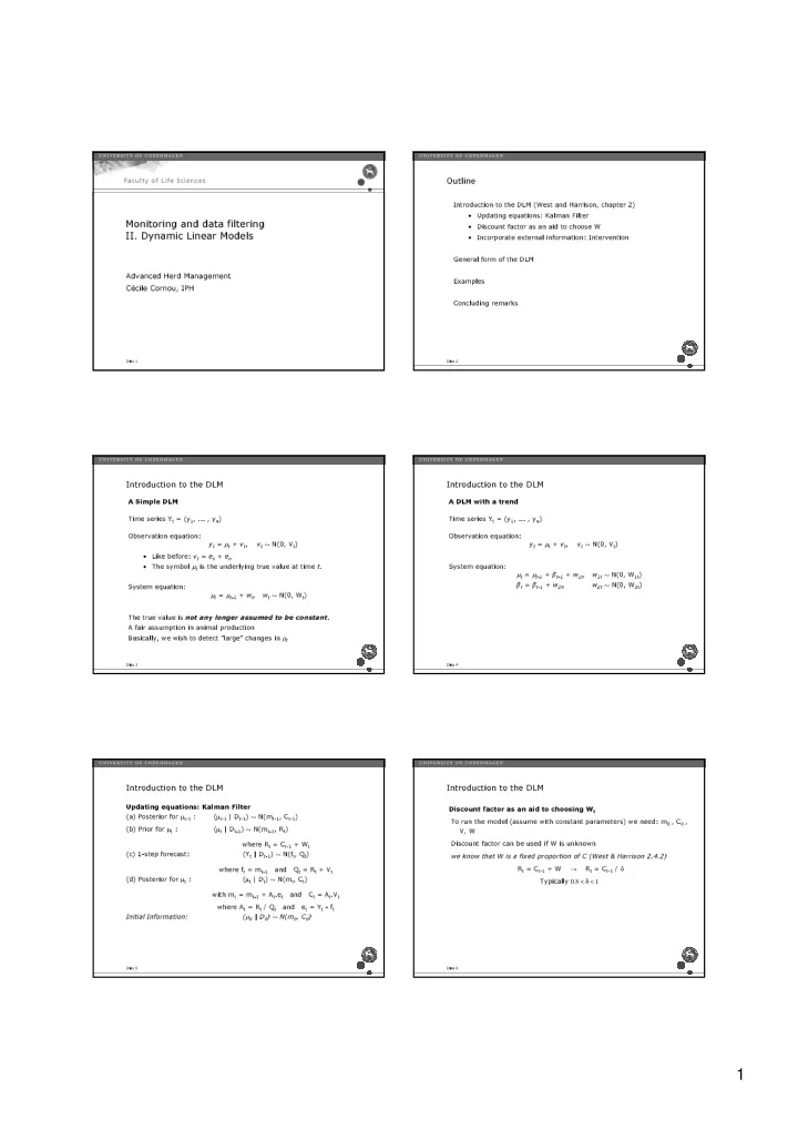
  1. Outline Introduction to the DLM (West and Harrison, chapter 2) • Updating equations: Kalman Filter Monitoring and data filtering • Discount factor as an aid to choose W II. Dynamic Linear Models • Incorporate external information: Intervention General form of the DLM Advanced Herd Management Examples Cécile Cornou, IPH Concluding remarks Dias 1 Dias 2 Introduction to the DLM Introduction to the DLM A Simple DLM A DLM with a trend Time series Y t = (y 1 , ... , y n ) Time series Y t = (y 1 , ... , y n ) Observation equation: Observation equation: y t = µ t + v t , v t ∼ N(0, V t ) y t = µ t + v t , v t ∼ N(0, V t ) • Like before: v t = e s + e o The symbol µ t is the underlying true value at time t . • System equation: µ t = µ t-1 + β t-1 + w 1t , w 1t ∼ N(0, W 1t ) β t = β t-1 + w 2t , w 2t ∼ N(0, W 2t ) System equation: µ t = µ t -1 + w t , w t ∼ N(0, W t ) The true value is not any longer assumed to be constant . A fair assumption in animal production Basically, we wish to detect ”large” changes in µ t Dias 3 Dias 4 Introduction to the DLM Introduction to the DLM Updating equations: Kalman Filter Discount factor as an aid to choosing W t (a) Posterior for µ t-1 : ( µ t-1 | D t-1 ) ∼ N(m t-1 , C t-1 ) (b) Prior for µ t : ( µ t | D t-1 ) ∼ N(m t-1 , R t ) To run the model (assume with constant parameters) we need: m 0 , C 0 , V , W where R t = C t-1 + W t Discount factor can be used if W is unknown (c) 1-step forecast: (Y t | D t-1 ) ∼ N(f t , Q t ) we know that W is a fixed proportion of C (West & Harrison 2.4.2) R t = C t-1 / δ where f t = m t-1 and Q t = R t + V t R t = C t-1 + W → (d) Posterior for µ t : ( µ t | D t ) ∼ N(m t , C t ) Typically 0.8 < δ < 1 with m t = m t-1 + A t .e t and C t = A t .V t where A t = R t / Q t and e t = Y t - f t ( µ 0 | D 0 ) ∼ N(m 0 , C 0 ) Initial Information: Dias 5 Dias 6 1

  2. Introduction to the DLM Introduction to the DLM Intervention - 1. Known effect Incorporate external information: intervention Types of external information: We want the model to adapt to the new known conditions Ex: Kurrit example from West and Harrison (2.3.2) 1. 1. Known effect, experienced before (ex: change in breed for Estimated mean after change: 286 (vs. 143) which we know the different performances) → We want the model to adapt to the new known conditions Expected change = 143 (286 – 143) • 2. Unknown effect (ex: wave of heat, introduction of new animals Uncertainty: from 80 (pessimistic) to 200 (optimistic) in a group) → We want the model to adapt to the new unknown conditions σ = 30 ( = (200 – 80) / 4) : 4 st.dev (95% interval) Variance associated (Uncertainty) = 30 2 = 900 (ω 10 | D 9 , S 9 ) ∼ N (143, 900) • 3. Unknown effect we want to measure (ex: change of feed composition, new veterinary treatments) Revised one-step ahead forecast: ( µ t | D t-1 ) ∼ N(m t-1 , R t ) → We want to measure the effect of a volontary change ( µ 10 | D 9 , S 9 ) ∼ N (286, 920) m 9 = 286 and R 10 = C 9 + W 10 = 20 + 900 = 920 Dias 7 Dias 8 Introduction to the DLM Introduction to the DLM Intervention - 2. Unknown effect (2/2) Intervention - 2. Unknown effect (1/2) In practice we can temporarily reduce the value of the discount factor so We want the model to adapt to the new unknown conditions the evolution variance increases Ex 1: wave of heat We put more weight on the new observations and ”forget about the past” We can not adjust because we do not know the exact effect Ex 2: introduction of new animals in a group Consider a method aimed to detect oestrus by monitoring animal behaviour Incoming animals may modify the behaviour of the group See also eating rank Here, intervention aimed to increase model adaptation to new behaviour so to avoid ”alarms” due to a known event Dias 9 Dias 10 Introduction to the DLM The general DLM Intervention - 3. Unknown effect Generalisation from the 1.order pol. Model We want to measure the effect of a volontary change • Simple, most widely used DLM Ex: A new feed is used and we want to estimate the associated change in • Matrix notation allows to present the DLM in a general form and to treat daily gain more complex cases We know that the new feed is used from time τ (0 < τ < n) y t = µ t + λ t I t + v t , v t ∼ N(0, V t ) Three examples of application µ t = µ t -1 + w t , w t ∼ N(0, W t ) • Monitoring activity level • Monitoring activity types (MPKF) With: • Monitoring eating behaviour λ t = 0 when t < τ I t : intervention effect that we want to measure λ t = 1 when t > τ Dias 11 Dias 12 2

  3. Modeling of the variable Monitoring Deviations from the model Dynamic Linear Models (DLMs) combined with Kalman Filter (KF) V-mask (parameters d and Ψ) Let Y t = ( y 1 , … , y n )’ be a vector of key figures observed at time t . Applied on the cumulative sum (cusum) of the standardized errors Let θ t = ( θ 1 , … , θ m )’ be a vector of parameters describing the system at time t. u t = e t /√Q t t C = ∑ u = u + c t t t t − 1 t = General form of the DLM 1 Observation Equation: Y t = F’ t θ t + ν t , ν t ~ N(0,V t ) System Equation: θ t = G t θ t-1 + ω t , ω t ~ N(0,W t ) DLM combined with Kalman Filter: estimate the underlying state vector θ t by its mean vector m t and its variance-covariance matrix C t . Tabular Cusum (parameters K and H) Elements from KF used in monitoring deviations: Create a cusum: accumulate u i , using a reference value (K) • f t : One step forecast mean • e t : One step forecast error (e t = Y t – f t ) Alarm when cusum exceeds a decision interval (H) • Q t : One step forecast variance Dias 13 Dias 14 Example 1. Oestrus Detection Monitoring activity level Oestrus Detection I (from day 4) • BPT (3 x / day) in the mating section Sow not inseminated Context Transfered to gestation section Development of Group housing in EU results of Council Directive 2001/88/EEC Difficulties identifying and accessing individual sow Oestrus Detection II (from day 21) Idea Store data in a chip and transmit info to the farmer’s PC • BPT (3 x / day) in the gestation section Sensor in the chip allows to monitor activity of the sow Golden Standard Assumption Detect whether activity pattern changes at onset of Body Activity of sows is expected to change around the onset of oestrus oestrus Objective Develop an automated oestrus detection method for group housed sows using sows’ acceleration measurements Weaning Transfer Acceleration measurements Method Use of Dynamic Linear Models to model the sows’ activity d0 d7 d10 d21 d30 BPT I BPT II Use of control methods that detects model deviations at the onset of oestrus Dias 15 Dias 16 Data collection Definition of the DLM Use hourly averages of the length of the acceleration vector Place, Animals, Housing and Feeding 2 + acc y 2 + acc z 2 ) • 1 production herd, March 2005 Y t = acc = √ (acc x µ • 5 sows in group of 100 ( ) F ' = G t = I θ = t 1 , 0 • 20 days   t t  0      Activity Measurements • Acceleration in 2 and 3 dimensions • Four measurements per second V t = unknow and constant • Transfer PC via Blue Tooth W t = 0 (In normal condition: no change in activity) Video Recordings • Four cameras used as web cam Model initialized by mean of Reference Analysis Oestrus Detection • Golden standard Model observations (Y t ) weighted by number of observations per hour Detect whether activity pattern changes at onset of oestrus Missing observation: e t =0 Dias 17 Dias 18 3

  4. Example 2. Illustration Monitoring sows’ activity types Daily Anoestrus Model Assumption Sow’s behaviour is affected by physiological state / illness Cusum Daily Oestrus • Oestrus: increase in activity • Lameness: walking V-mask Accelerometer: measured any time / during whole reproductive cycle Objective Develop a method that automatically classify sows’ activity types Tabular Cusum Model selected activity types using DLM Classify each activity type using a Multi Process Kalman Filter Dias 19 Dias 20 Acceleration data Time series and activity types Activity types Extracts from time series of acceleration are associated to five activity types • Feeding (FE) 3 dimensions: X,Y, Z • Rooting (RO) 2 + acc y 2 + acc z 2 ) • Walking (WA) ACC = √ (acc x • Lying sternally (LS) • Lying Laterally (LL) Two data sets Activity filled whole data set / no overlapping Learning data set: 10 minutes of each activity type X Estimate the model parameters Y Test data set: 10 x 2 minutes of each activity type Z Implement the classification method ACC Dias 21 Dias 22 Modeling each activity type Classification method Use averages per second of acceleration data Multi Process Kalman Filter of class I µ t At time t :   π π θ = 2 2 s G t = I   F t = t t '  1 , sin   , cos    t t T T         Each DLM is analysed using the updating equations of the Kalman Filter:   c         t • One step forecast mean f t   • One step forecast variance Q t Model includes a periodic movement – cyclic components V and W: estimated using the EM algorithm Posterior Probabilities are estimated for each DLM Learning data set p i ∝ φ i × p 1 i ( ) ( ) ( ) t t t − 20 DLMs 5 activities x 4 axes (X, Y, Z, ACC) Dias 23 Dias 24 4

Download Presentation
Download Policy: The content available on the website is offered to you 'AS IS' for your personal information and use only. It cannot be commercialized, licensed, or distributed on other websites without prior consent from the author. To download a presentation, simply click this link. If you encounter any difficulties during the download process, it's possible that the publisher has removed the file from their server.

Recommend


More recommend