[PDF] - 1 Being Normal, Simultaneously Maximizing Likelihood with Uniform PDF Document

SLIDE 1

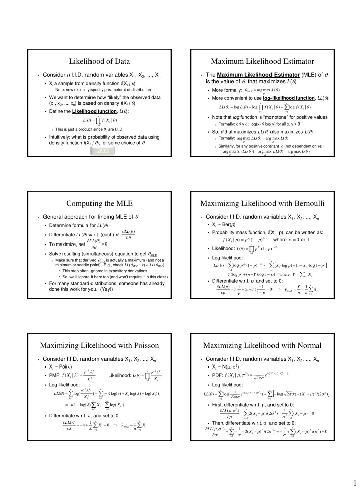
1 Likelihood of Data

Consider n I.I.D. random variables X1, X2, ..., Xn
Xi a sample from density function f(Xi | )
Note: now explicitly specify parameter  of distribution
We want to determine how “likely” the observed data

(x1, x2, ..., xn) is based on density f(Xi | )

Define the Likelihood function, L():
This is just a product since Xi are I.I.D.
Intuitively: what is probability of observed data using

density function f(Xi | ), for some choice of 





n i i

X f L

1

) | ( ) (  

Demo

Maximum Likelihood Estimator

The Maximum Likelihood Estimator (MLE) of ,

is the value of  that maximizes L()

More formally:
More convenient to use log-likelihood function, LL():
Note that log function is “monotone” for positive values
Formally: x ≤ y  log(x) ≤ log(y) for all x, y > 0
So,  that maximizes LL() also maximizes L()
Formally:
Similarly, for any positive constant c (not dependent on ):

) ( max arg  



L

MLE 

 

 

  

n i i n i i

X f X f L LL

1 1

) | ( log ) | ( log ) ( log ) (     ) ( max arg ) ( max arg  

 

L LL  ) ( max arg ) ( max arg )) ( ( max arg   

  

L LL LL c   

Computing the MLE

General approach for finding MLE of 
Determine formula for LL()
Differentiate LL() w.r.t. (each)  :
To maximize, set
Solve resulting (simultaneous) equation to get MLE
Make sure that derived is actually a maximum (and not a

minimum or saddle point). E.g., check LL(MLE ) < LL(MLE)

This step often ignored in expository derivations
So, we’ll ignore it here too (and won’t require it in this class)
For many standard distributions, someone has already

done this work for you. (Yay!)

    ) ( LL ) (      LL

MLE

 ˆ

Maximizing Likelihood with Bernoulli

Consider I.I.D. random variables X1, X2, ..., Xn
Xi ~ Ber(p)
Probability mass function, f(Xi | p), can be written as:
Likelihood:
Log-likelihood:
Differentiate w.r.t. p, and set to 0:

1 ) 1 ( ) | (

1

r

where   

 i x x i

x p p p X f

i i



 

 

n i X X

i i

p p L

1 1

) 1 ( ) (

 

 

  

     

n i i i n i X X

p X p X p p LL

i i

1 1 1

) 1 log( ) 1 ( ) (log ) ) 1 ( log( ) (

 

    

n i i

X Y p Y n p Y

1

where ) 1 log( ) ( ) (log





          

n i i MLE

X n n Y p p Y n p Y p p LL

1

1 1 1 ) ( 1 ) (

Maximizing Likelihood with Poisson

Consider I.I.D. random variables X1, X2, ..., Xn
Xi ~ Poi(l)
PMF:

Likelihood:

Log-likelihood:
Differentiate w.r.t. l, and set to 0:

! ) | (

i x i

x e X f

i

l l

l 





 



n i i X

X e L

i

1

! ) ( l 

l

 

 

  

    

n i i i n i i X

X X e X e LL

i

1 1

) ! log( ) log( ) log( ) ! log( ) ( l l l 

l

 

 

       

n i i MLE n i i

X n X n LL

1 1

1 1 ) ( l l l l

 

 

   

n i i n i i

X X n

1 1

) ! log( ) log(l l

Maximizing Likelihood with Normal

Consider I.I.D. random variables X1, X2, ..., Xn
Xi ~ N(m, 2)
PDF:
Log-likelihood:
First, differentiate w.r.t. m, and set to 0:
Then, differentiate w.r.t. , and set to 0:

) 2 /( ) ( 2

2 2

2 1

) , | (

 m

 

 m

 



i

X i

e X f

 

 

   

    

n i i n i X

X e LL

i

1 2 2 1 ) 2 /( ) (

) 2 /( ) ( ) 2 log( ) log( ) (

2 2

2 1

 m   

 m

 

) ( 1 ) 2 /( ) ( 2 ) , (

1 2 1 2 2

      

 

  n i i n i i

X X LL m   m m  m ) /( ) ( ) 2 /( ) ( 2 1 ) , (

1 3 2 1 3 2 2

          

 

  n i i n i i

X n X LL  m   m    m

SLIDE 2

2 Being Normal, Simultaneously

Now have two equations, two unknowns:
First, solve for mMLE:
Then, solve for 2MLE:
Note: mMLE unbiased, but 2

MLE biased (same as MOM)

) ( 1

1 2

 



 n i i

X m  ) /( ) (

1 3 2

   



 n i i

X n  m 

  

  

     

n i i MLE n i i n i i

X n n X X

1 1 1 2

1 ) ( 1 m m m 

 

 

      

n i i n i i

X n X n

1 2 2 1 3 2

) ( ) /( ) ( m   m 





 

n i MLE i

X n

MLE

1 2 2

) ( 1 m 

Maximizing Likelihood with Uniform

Consider I.I.D. random variables X1, X2, ..., Xn
Xi ~ Uni(a, b)
PDF:
Likelihood:
Constraint a < x1, x2, …, xn < b makes differentiation tricky
Intuition: want interval size (b – a) to be as small as possible to

maximize likelihood function for each data point

But need to make sure all observed data contained in interval
If all observed data not in interval, then L() = 0
Solution: aMLE = min(x1, …, xn) bMLE = max(x1, …, xn)

       

       



therwise

,..., , ) (

2 1

1

b x x x a L

n

a b

        



therwise

) , | (

1

b x a b a X f

i i

a b

Understanding MLE with Uniform

Consider I.I.D. random variables X1, X2, ..., Xn
Xi ~ Uni(0, 1)
Observe data:
0.15, 0.20, 0.30, 0.40, 0.65, 0.70, 0.75

Likelihood: L(a,1)

a L(a,1)

Likelihood: L(0, b)

b L(0, b)

Once Again, Small Samples = Problems

How do small samples effect MLE?
In many cases, = sample mean
Unbiased. Not too shabby…
As seen with Normal,
Biased. Underestimates for small n (e.g., 0 for n = 1)
As seen with Uniform, aMLE ≥ a and bMLE ≤ b
Biased. Problematic for small n (e.g., a = b when n = 1)
Small sample phenomena intuitively make sense:
Maximum likelihood  best explain data we’ve seen
Does not attempt to generalize to unseen data





n i i MLE

X n

1

1 m





 

n i MLE i

X n

MLE

1 2 2

) ( 1 m 

Properties of MLE

Maximum Likelihood Estimators are generally:
Consistent: for  > 0
Potentially biased (though asymptotically less so)
Asymptotically optimal
Has smallest variance of “good” estimators for large samples
Often used in practice where sample size is large

relative to parameter space

But be careful, there are some very large parameter spaces
Joint distributions of several variables can cause problems
Parameter space grows exponentially
Parameter space for 10 dependent binary variables  210

1 ) | ˆ (| lim   

 

   P

n

Maximizing Likelihood with Multinomial

Consider I.I.D. random variables Y1, Y2, ..., Yn
Yk ~ Multinomial(p1, p2, ..., pm), where
Xi = number of trials with outcome i where
PDF:
Log-likelihood:
Account for constraint when differentiating LL()
Use Lagrange multipliers (drop non-pi terms):

 

 

  

m i i i m i i

p X X n LL

1 1

) log( ) ! log( ) ! log( ) (





m i i 1

1 p

m

x m x x m m m

p p p p p X X f

x x x n

... ) ,..., | ,..., (

2 1

2 1 2 1 1 1

! ! ! !   







m i i 1

n X





m i i 1

1 p ) 1 ( ) log( ) (

1 1

  

 

  m i i m i i i

p p X A l 

Joseph-Louis Lagrange (1736-1813)

Rock on, dog!

SLIDE 3

3 Home on Lagrange

Want to maximize:
Differentiate w.r.t. each pi, in turn:
Solve for l, noting and :
Substitute l into pi, yielding:
Intuitive result: probability pi = proportion of outcome i

) 1 ( ) log( ) (

1 1

  

 

  m i i m i i i

p p X A l  l l 

i i i i i

X p p X p A         1 ) (





m i i 1

n X





m i i 1

1 p

n n X p

m i i m i i

       



 

l l l 1

1 1

n X p

i i 

When MLE’s Attack!

Consider 6-sided die
X ~ Multinomial(p1, p2, p3, p4, p5, p6)
Roll n = 12 times
Result: 3 ones, 2 twos, 0 threes, 3 fours, 1 fives, 3 sixes
Consider MLE for pi:
p1 = 3/12, p2 = 2/12, p3 = 0/12, p4 = 3/12, p5 = 1/12, p6 = 3/12
Based on estimate, infer that you will never roll a three
Do you really believe that?
Frequentist: Need to roll more! Probability = frequency in limit
Bayesian: Have prior beliefs of probability, even before any rolls!

Need a Volunteer

So good to see you again!

Two Envelopes

I have two envelopes, will allow you to have one
One contains $X, the other contains $2X
Select an envelope
Open it!
Now, would you like to switch for other envelope?
To help you decide, compute E[$ in other envelope]
Let Y = $ in envelope you selected
Before opening envelope, think either equally good
So, what happened by opening envelope?
And does it really make sense to switch?

Y Y E

Y 4 5 2 1 2 2 1

2 ] envelope

ther

in $ [     