1 Geometric Interpretation: Cubic Why Polar Forms? Why Polar - - PDF document

SLIDE 1

1

Foundations of Computer Graphics Foundations of Computer Graphics (Spring 2012) (Spring 2012)

CS 184, Lecture 13: Curves 2

http://inst.eecs.berkeley.edu/~cs184

Outline of Unit Outline of Unit

• Bezier curves (last time)
• deCasteljau algorithm, explicit, matrix (last time)
• Polar form labeling (blossoms)
• B-spline curves
• Not well covered in textbooks (especially as taught

here). Main reference will be lecture notes. If you do want a printed ref, handouts from CAGD, Seidel

Idea of Blossoms/Polar Forms Idea of Blossoms/Polar Forms

• (Optional) Labeling trick for control points and intermediate

deCasteljau points that makes thing intuitive

• E.g. quadratic Bezier curve F(u)
• Define auxiliary function f(u1,u2) [number of args = degree]
• Points on curve simply have u1=u2 so that F(u) = f(u,u)
• And we can label control points and deCasteljau points not
• n curve with appropriate values of (u1,u2 )

f(0,0) = F(0) f(1,1) = F(1) f(0,1)=f(1,0) f(u,u) = F(u)

Idea of Blossoms/Polar Forms Idea of Blossoms/Polar Forms

• Points on curve simply have u1=u2 so that F(u) = f(u,u)
• f is symmetric f(0,1) = f(1,0)
• Only interpolate linearly between points with one arg different
• f(0,u) = (1-u) f(0,0) + u f(0,1) Here, interpolate f(0,0) and f(0,1)=f(1,0)

00 01 11

F(u) = f(uu) = (1-u)2 P0 + 2u(1-u) P1 + u2 P2 1-u 1-u u u 1-u u

0u 1u uu

f(0,0) = F(0) f(1,1) = F(1) f(0,1)=f(1,0) f(u,u) = F(u)

Geometric interpretation: Quadratic Geometric interpretation: Quadratic

u u u 1-u 1-u 00 01=10 11 0u 1u uu

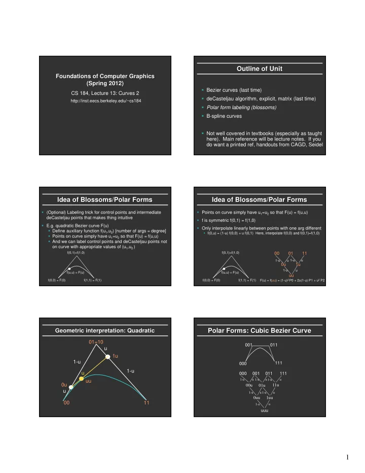
Polar Forms: Cubic Bezier Curve Polar Forms: Cubic Bezier Curve

000 001 011 111 000 001 011 111

1-u u u u 1-u 1-u

00u 01u 11u

1-u u u 1-u

0uu 1uu

1-u u

uuu

SLIDE 2

2 Geometric Interpretation: Cubic

00u 0u1 u11 0uu uu1 uuu 000 111 001 011

Why Polar Forms? Why Polar Forms?

• Simple mnemonic: which points to interpolate and

how in deCasteljau algorithm

• Easy to see how to subdivide Bezier curve (next)

which is useful for drawing recursively

• Generalizes to arbitrary spline curves (just label

control points correctly instead of 00 01 11 for Bezier)

• Easy for many analyses (beyond scope of course)

Subdividing Bezier Curves Subdividing Bezier Curves

Drawing: Subdivide into halves (u = ½) Demo: hw4.exe

• Recursively draw each piece
• At some tolerance, draw control polygon
• Trivial for Bezier curves (from deCasteljau algorithm): hence

widely used for drawing

Why specific labels/ control points on left/right?

• How do they follow from deCasteljau?

000 001 011 111 000 00u 0uu uuu uuu uu1 u11 111

Geometrically

00½ 0½1 ½11 0½½ ½½1 ½½½ 000 111 001 011

Geometrically

00½ 0½1 ½11 0½½ ½½1 ½½½ 000 111 001 011

Subdivision in Subdivision in deCasteljau deCasteljau diagram diagram

000 001 011 111 000 001 011 111

1-u u u u 1-u 1-u

00u 01u 11u

1-u u u 1-u

0uu 1uu

1-u u

uuu

Left part of Bezier curve (000, 00u, 0uu, uuu) Always left edge of deCasteljau pyramid Right part of Bezier curve (uuu, 1uu, 11u, 111) Always right edge of deCasteljau pyramid These (interior) points don’t appear in subdivided curves at all

SLIDE 3

3

Summary for HW 2 Summary for HW 2

• Bezier2 (Bezier discussed last time)
• Given arbitrary degree Bezier curve, recursively

subdivide for some levels, then draw control polygon

hw4.exe

• Generate deCasteljau diagram; recursively call a routine

with left edge and right edge of this diagram

• You are given some code structure; you essentially just

need to compute appropriate control points for left, right

DeCasteljau DeCasteljau: Recursive Subdivision : Recursive Subdivision

• DeCasteljau (from last lecture) for midpoint
• Followed by recursive calls using left, right parts

Outline of Unit Outline of Unit

• Bezier curves (last time)
• deCasteljau algorithm, explicit, matrix (last time)
• Polar form labeling (blossoms)
• B-spline curves
• Not well covered in textbooks (especially as taught

here). Main reference will be lecture notes. If you do want a printed ref, handouts from CAGD, Seidel

Bezier: Disadvantages Bezier: Disadvantages

• Single piece, no local control (move a control point,

whole curve changes) hw4.exe

• Complex shapes: can be very high degree, difficult
• In practice, combine many Bezier curve segments
• But only position continuous at join since Bezier curves

interpolate end-points (which match at segment boundaries)

• Unpleasant derivative (slope) discontinuities at end-points
• Can you see why this is an issue?

B B-

• Splines

Splines

• Cubic B-splines have C2 continuity, local control
• 4 segments / control point, 4 control

points/segment

• Knots where two segments join: Knotvector
• Knotvector uniform/non-uniform (we only consider

uniform cubic B-splines, not general NURBS)

Knot: C2 continuity deBoor points

Demo: hw4.exe

Polar Forms: Cubic Polar Forms: Cubic Bspline Bspline Curve Curve

• 2 –1 0

–1 0 1 0 1 2 1 2 3

• Labeling little different from in Bezier curve
• No interpolation of end-points like in Bezier
• Advantage of polar forms: easy to generalize

Uniform knot vector:

• 2, -1, 0, 1, 2 ,3

Labels correspond to this

SLIDE 4

4

deCasteljau deCasteljau: Cubic B : Cubic B-

• Splines

Splines

• Easy to generalize using

polar-form labels

• Impossible remember

without

• 2 –1 0

–1 0 1 0 1 2 1 2 3

• 2 -1 0
• 1 0 1

0 1 2 1 2 3

• 1 0 u

0 1 u 1 2 u

? ? ? ? ? ?

deCasteljau deCasteljau: Cubic B : Cubic B-

• Splines

Splines

• Easy to generalize using

polar-form labels

• Impossible remember

without

• 2 –1 0

–1 0 1 0 1 2 1 2 3

• 2 -1 0
• 1 0 1

0 1 2 1 2 3

• 1 0 u

0 1 u 1 2 u

1-u/3 (1-u)/3 (2+u)/3 (2-u)/3 (1+u)/3 u/3

0 u u 1 u u

? ? ? ?

deCasteljau deCasteljau: Cubic B : Cubic B-

• Splines

Splines

• Easy to generalize using

polar-form labels

• Impossible remember

without

• 2 –1 0

–1 0 1 0 1 2 1 2 3

• 2 -1 0
• 1 0 1

0 1 2 1 2 3

• 1 0 u

0 1 u 1 2 u

1-u/3 (1-u)/3 (2+u)/3 (2-u)/3 (1+u)/3 u/3

0 u u 1 u u

(1-u)/2 (1+u)/2 1-u/2 u/2

u u u

1-u u

Explicit Formula (derive as exercise) Explicit Formula (derive as exercise)

• 2 -1 0
• 1 0 1

0 1 2 1 2 3

• 1 0 u

0 1 u 1 2 u

1-u/3 (1-u)/3 (2+u)/3 (2-u)/3 (1+u)/3 u/3

0 u u 1 u u

(1-u)/2 (1+u)/2 1-u/2 u/2

u u u

1-u u

3 2

1 ( ) [ 1] 2 3 P P F u u u u P P

M

            

1 3 3 1 3 6 3 3 3 1 4 1

1 6

M

               



P0 P1 P2 P3

Summary of HW 2 Summary of HW 2

• BSpline Demo hw4.exe
• Arbitrary number of control points / segments
• Do nothing till 4 control points (see demo)
• Number of segments = # cpts – 3
• Segment A will have control pts A,A+1,A+2,A+3
• Evaluate Bspline for each segment using 4 control

points (at some number of locations, connect lines)

• Use either deCasteljau algorithm (like Bezier) or

explicit form [matrix formula on previous slide]

• Questions?