1.8 Intro to Linear Transformations McDonald Fall 2018, MATH 2210Q, - PDF document

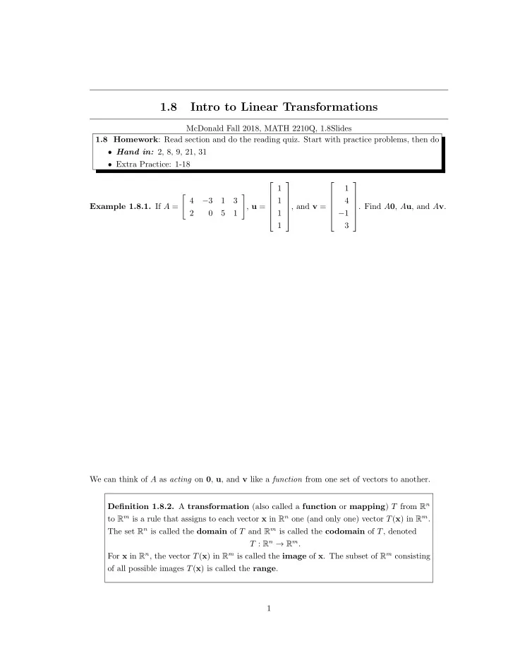
1.8 Intro to Linear Transformations McDonald Fall 2018, MATH 2210Q, 1.8Slides 1.8 Homework : Read section and do the reading quiz. Start with practice problems, then do ❼ Hand in: 2, 8, 9, 21, 31 ❼ Extra Practice: 1-18     1 1 � �     4 − 3 1 3 1 4     Example 1.8.1. If A = , u = , and v = . Find A 0 , A u , and A v .     2 0 5 1 1 − 1         1 3 We can think of A as acting on 0 , u , and v like a function from one set of vectors to another. Definition 1.8.2. A transformation (also called a function or mapping ) T from R n to R m is a rule that assigns to each vector x in R n one (and only one) vector T ( x ) in R m . The set R n is called the domain of T and R m is called the codomain of T , denoted T : R n → R m . For x in R n , the vector T ( x ) in R m is called the image of x . The subset of R m consisting of all possible images T ( x ) is called the range . 1

Remark 1.8.3. In this section, we will focus on mappings associated to matrix multiplication . For simplicity, we sometimes denote this matrix transformation by x �→ A x .       1 − 3 3 3 � � 2 Example 1.8.4. Let A =  , u = , b =  , c =  , 3 5 2 2        − 1   − 1 7 − 5 5 and define a transformation T : R 2 → R 3 by T ( x ) = A x . (a) Write T ( x ) as a vector. (b) Find T ( u ), the image of u under the transformation T . (c) Find an x in R 2 such that T ( x ) = b . Is there more than one? (d) Determine if c is in the range of T . 2

  1 0 0 Example 1.8.5. Let A =  and describe x �→ A x . 0 1 0    0 0 0 Remark 1.8.6. The map in Example 1.8.5 is called a projection map. � � � � � � 1 2 0 1 Example 1.8.7. Let A = , and T ( x ) = A x . Find the images of u = , v = , 0 1 1 0 � � 1 and u + v = under T , and use this to describe T geometrically. 1 Remark 1.8.8. The map in Example 1.8.7 is called a shear transformation . 3

Definition 1.8.9. A transformation T is called linear if (i) T ( u + v ) = T ( u ) + T ( v ) for all u , v in the domain of T ; (ii) T ( c u ) = cT ( u ) for all scalars c and u in the domain of T . Remark 1.8.10. The properties of A x Section 1.4 show that when T is a matrix transformation , T is a linear transformation. Not all transformations are linear, however. Proposition 1.8.11. If T is a linear transformation, then T ( 0 ) = 0 , and T ( c u + d v ) = cT ( u ) + dT ( v ) for all vectors u , v in the domain of T , and all scalars c, d . Remark 1.8.12. If T satisfies the second property above, then it is as linear transformation. Repeated application of this property gives T ( c 1 u 1 + · · · + c n v n ) = c 1 T ( u 1 ) + · · · + c n T ( v n ) In physics and engineering, this is called a superposition principle . Example 1.8.13. Given a scalar r ≥ 0, define T : R 2 → R 2 by T ( x ) = r x . Prove T is a linear transformation, and describe it geometrically. Remark 1.8.14. In Example 1.8.12, the linear transformation T is called a contraction when 0 < r < 1 and a dilation when r > 1. 4

� � � � � � 0 − 1 3 1 Example 1.8.15. Let A = , and T ( x ) = A x . Find the images of u = , v = , 1 0 1 2 � � 4 and u + v = under T , and use this to describe T geometrically. 3 5

1.8.1 Additional Thoughts and Problems 6