Outline Types of transformations and invariance Scale invariance - - PDF document

Lecture 13: Local invariant features

Tuesday, Oct 30

• Prof. Kristen Grauman

Outline

• Types of transformations and invariance

– Scale invariance

• Local features: detectors and descriptors

– SIFT

• What would we like our image descriptions

to be invariant to?

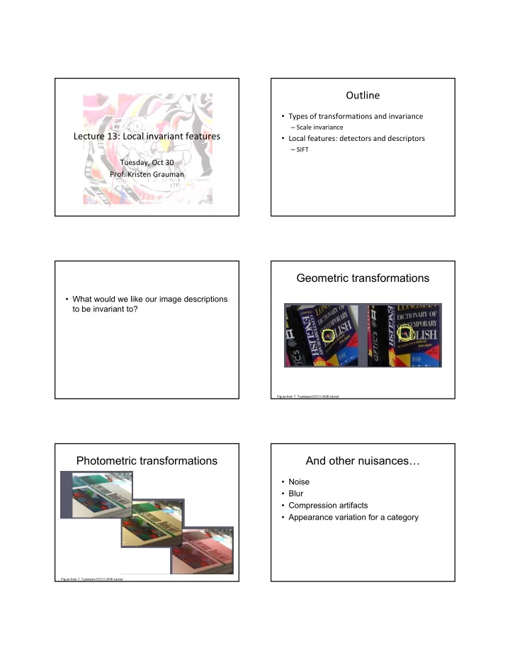
Geometric transformations

Figure from T. Tuytelaars ECCV 2006 tutorial

Photometric transformations

Figure from T. Tuytelaars ECCV 2006 tutorial

And other nuisances…

• Noise
• Blur
• Compression artifacts
• Appearance variation for a category

Classes of transformations

• Euclidean/rigid:

Translation + rotation

• Similarity: Translation +

rotation + uniform scale

• Affine: Similarity + shear

– Valid for orthographic camera, locally planar

• bject
• (Projective: Affine +

projective warps)

• Photometric: affine

intensity change

– I -> aI + b

Similarity transformation Translation and Scaling Translation Affine transformation Projective transformation

Exhaustive search

A multi-scale approach

Slide from T. Tuytelaars ECCV 2006 tutorial

Exhaustive search

A multi-scale approach

Slide from T. Tuytelaars ECCV 2006 tutorial

Exhaustive search

A multi-scale approach

Slide from T. Tuytelaars ECCV 2006 tutorial

Exhaustive search

A multi-scale approach

Slide from T. Tuytelaars ECCV 2006 tutorial

Key idea of invariance

Slide adapted from T. Tuytelaars ECCV 2006 tutorial

We want to extract the patches from each image independently.

Invariant local features

Subset of local feature types designed to be invariant to

– Scale – Translation – Rotation – Affine transformations – Illumination

1) Detect distinctive interest points

2) Extract invariant descriptors

[Mikolajczyk & Schmid, Matas et al., Tuytelaars & Van Gool, Lowe, Kadir et al.,… ]

x 1 x 2 … x d y1 y2 … yd

(Good) invariant local features

• Reliably detected
• Distinctive
• Robust to noise, blur, etc.
• Description normalized properly

Interest points: From stereo to recognition

• Feature detectors previously used for

stereo, motion tracking

• Now also for recognition

– Schmid & Mohr 1997

• Harris corners to select interest points
• Rotationally invariant descriptor of local image

regions

• Identify consistent clusters of matched features

to do recognition “flat” region: no change in all directions “edge”: no change along the edge direction “corner”: significant change in all directions

C.Harris, M.Stephens. “A Combined Corner and Edge Detector”. 1988

Review: corner detection as an interest

• perator

[Slide credit: Darya Frolova and Denis Simakov]

Review: Harris Detector Workflow Review: Harris Detector Workflow

Compute corner response R

Review: Harris Detector Workflow

Find points with large corner response: R>threshold

Review: Harris Detector Workflow

Take only the points of local maxima of R

Review: Harris Detector Workflow

Harris Detector

• Rotation invariance

Ellipse rotates but its shape (i.e. eigenvalues) remains the same Corner response R is invariant to image rotation

But, for corner detection we must search windows at a pre-determined scale.

Scale space (Witkin 83)

larger

Gaussian filtered 1d signal first derivative peaks

Adapted from Steve Seitz, UW

x contours of f’’ = 0 in scale-space

Scale space

Scale space insights:

• edge position may shift with increasing scale (σ)
• two edges may merge with increasing scale

(edges can disappear)

• an edge may not split into two with increasing

scale (new edges do not appear)

Scale Invariant Detection

• Consider regions of different sizes around a

point

• At the right scale, regions of corresponding

content will look the same in both images

[Slides by Darya Frolova and Denis Simakov]

Scale Invariant Detection

• The problem: how do we choose

corresponding circles independently in each image?

Scale Invariant Detection

• Solution:

– Design a function on the region (circle), which is “scale invariant” (the same for corresponding regions, even if they are at different scales)

Example: average intensity. For corresponding regions (even of different sizes) it will be the same. scale = 1/2

– For a point in one image, we can consider it as a function of region size (circle radius) f

region size Image 1

f

region size Image 2

Scale Invariant Detection

• Common approach:

scale = 1/2

f

region size Image 1

f

region size Image 2

Take a local maximum of this function

Observation: region size, for which the maximum is achieved, should be invariant to image scale.

s1 s2

Important: this scale invariant region size is found in each image independently!

Scale Invariant Detection

[Images from T. Tuytelaars]

Following example was created by T. Tuytelaars, ECCV 2006 tutorial

Scale Invariant Detection

• A “good” function for scale detection:

has one stable sharp peak

f

region size

bad

f

region size

bad

f

region size

Good !

• For usual images: a good function would be a
• ne which responds to contrast (sharp local

intensity change)

Scale space

Scale space insights:

• edge position may shift with increasing scale (σ)
• two edges may merge with increasing scale

(edges can disappear)

• an edge may not split into two with increasing

scale (new edges do not appear) What could be an approximation of an image’s scale space?

Scale invariant detection

Requires a method to repeatably select points in location and scale:

– Only reasonable scale-space kernel is a Gaussian (Koenderink, 1984; Lindeberg, 1994) – An efficient choice is to detect peaks in the difference

• f Gaussian pyramid (Burt & Adelson, 1983; Crowley

& Parker, 1984) – Difference-of-Gaussian is a close approximation to Laplacian

Slide adapted from David Lowe, UBC

Scale selection principle

• Intrinsic scale is the scale at which

normalized derivative assumes a maximum -- marks a feature containing interesting structure. (T. Lindeberg ’94)

Maxima/minima of Laplacian

Scale Invariant Detection

2 2 2

1 2 2

( , , )

x y

G x y e

σ πσ

σ

+ −

=

( )

2

( , , ) ( , , )

xx yy

L G x y G x y σ σ σ = + ( , , ) ( , , ) DoG G x y k G x y σ σ = − Kernels:

where Gaussian (Laplacian) (Difference of Gaussians)

Kernel Image f = ∗

[Slide by Darya Frolova and Denis Simakov]

Scale space images: repeatedly convolve with Gaussian Adjacent Gaussian images subtracted

SIFT: Key point localization

n Detect maxima and minima

• f difference-of-Gaussian in

scale space

n Then reject points with low

contrast (threshold)

n Eliminate edge responses

(use ratio of principal curvatures)

Candidate keypoints: list of (x,y,σ)

Adapted from David Lowe, UBC

SIFT: Example of keypoint detection

Threshold on value at DOG peak and on ratio of principle curvatures (Harris approach)

(a) 233x189 image (b) 832 DOG extrema (c) 729 left after peak value threshold (d) 536 left after testing ratio of principle curvatures

Slide from David Lowe, UBC

Scale Invariant Detectors

K.Mikolajczyk, C.Schmid. “Indexing Based on Scale Invariant Interest Points”. ICCV 2001

• Experimental evaluation of detectors

w.r.t. scale change

Repeatability rate:

# correspondences # possible correspondences

Scale Invariant Detection: Summary

• Given: two images of the same scene with a

large scale difference between them

• Goal: find the same interest points

independently in each image

• Solution: search for maxima of suitable

functions in scale and in space (over the image)

Affine Invariant Detection

• Above we considered:

Similarity transform (rotation + uniform scale)

• Now we go on to:

Affine transform (rotation + non-uniform scale)

Affine Invariant Detection

• Intensity-based regions (IBR):

– Start from a local intensity extrema – Consider intensity profile along rays – Select maximum of invariant function f(t) along each ray – Connect local maxima – Fit an ellipse

T.Tuytelaars, L.V.Gool. “Wide Baseline Stereo Matching Based on Local, Affinely Invariant Regions”. BMVC 2000.

Affine Invariant Detection

Matas et al. Robust Wide Baseline Stereo from Maximally Stable Extremal Regions. BMVC 2002.

• Maximally Stable Extremal Regions

(MSER) – Threshold image intensities: I > I0 – Extract connected components (“Extremal Regions”) – Seek extremal regions that remain “Maximally Stable” under range of thresholds

Point Descriptors

• We know how to detect points
• Next question:

How to describe them for matching?

?

Point descriptor should be:

• 1. Invariant
• 2. Distinctive

Rotation Invariant Descriptors

• Harris corner response measure:

depends only on the eigenvalues of the matrix M

C.Harris, M.Stephens. “A Combined Corner and Edge Detector”. 1988

Rotation Invariant Descriptors

• Find local orientation

Dominant direction of gradient

• Rotate description relative to dominant
• rientation

1 K.Mikolajczyk, C.Schmid. “Indexing Based on Scale Invariant Interest Points”. ICCV 2001 2 D.Lowe. “Distinctive Image Features from Scale-Invariant Keypoints”. Accepted to IJCV 2004

Scale Invariant Descriptors

• Use the scale determined by detector to

compute descriptor in a normalized frame

[Images from T. Tuytelaars]

SIFT descriptors: Select canonical orientation

n Create histogram of local

gradient directions computed at selected scale

n Assign canonical orientation

at peak of smoothed histogram

n Each key specifies stable 2D

coordinates (x, y, scale,

• rientation)

2π

Slide by David Lowe, UBC

SIFT descriptors: vector formation

n Thresholded image gradients are sampled over 16x16

array of locations in scale space

n Create array of orientation histograms n 8 orientations x 4x4 histogram array = 128 dimensions

Slide by David Lowe, UBC

SIFT properties

• Invariant to

– Scale – Rotation

• Partially invariant to

– Illumination changes – Camera viewpoint – Occlusion, clutter

SIFT matching and recognition

n Index descriptors n Generalized Hough transform: vote for object poses n Refine with geometric verification: affine fit, check for

agreement between image features and model

SIFT Features

Adapted from David Lowe, UBC

Value of local (invariant) features

• Complexity reduction via selection of

distinctive points

• Describe images, objects, parts without

requiring segmentation

– Local character means robustness to clutter,

• cclusion
• Robustness: similar descriptors in spite of

noise, blur, etc.

Coming up

• Problem set 3 due 11/13

– Stereo matching – Local invariant feature indexing

• Thursday: image indexing with bags of words

– Read Video Google paper