1/31/2007 Massachusetts Institute of Technology Context Hybrid - - PDF document

1 31 2007
SMART_READER_LITE
LIVE PREVIEW

1/31/2007 Massachusetts Institute of Technology Context Hybrid - - PDF document

1/31/2007 Massachusetts Institute of Technology Context Hybrid Systems Hybrid discrete-continuous models are convenient for many systems Active Estimation for Switching Failure-prone components (Funiak03, Dearden02) Piloted


slide-1
SLIDE 1

1/31/2007 1

January 31, 2007

Massachusetts Institute of Technology

Active Estimation for Switching Linear Dynamic Systems

Lars Blackmore, Senthooran Rajamanoharan and Brian Williams

2

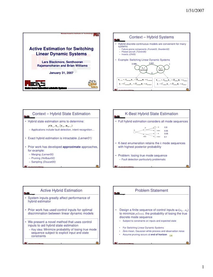
Context – Hybrid Systems

  • Hybrid discrete-continuous models are convenient for many

systems

– Failure-prone components (Funiak03, Dearden02) – Piloted aircraft (Tomlin06) – Insects (Oh05)

  • Example: Switching Linear Dynamic Systems

xd,t= nominal xd,t= failed 0.001 0.999 1

nominal nominal , nominal 1 ,

υ + + =

+ t t c t c

B A u x x

failure failure , failure 1 ,

υ + + =

+ t t c t c

B A u x x

nominal nominal , nominal

ω + + =

t t c t

D C u x y

failure failure , failure

ω + + =

t t c t

D C u x y

3

Context – Hybrid State Estimation

  • Hybrid state estimation aims to determine:

– Applications include fault detection, intent recognition…

  • Exact hybrid estimation is intractable (Lerner01)
  • Prior work has developed approximate approaches,

for example:

– Merging (Lerner00) – Pruning (Hofbaur02) – Sampling (Doucet00)

) , | , (

1 : : 1 , , − T T t d t c

p u y x x

4

K-Best Hybrid State Estimation

  • Full hybrid estimation considers all mode sequences
  • K-best enumeration retains the k mode sequences

with highest posterior probability

  • Problem: losing true mode sequence

– Fault detection particularly problematic

  • k
  • k

failed

  • k

failed failed

  • k

0.8 0.05 0.05 0.1

5

Active Hybrid Estimation

  • System inputs greatly affect performance of

hybrid estimator

  • Prior work has used control inputs for optimal

discrimination between linear dynamic models

  • We present a novel method that uses control

inputs to aid hybrid state estimation

– Key idea: Minimize probability of losing true mode

sequence subject to explicit input and state constraints

6

Problem Statement

  • Design a finite sequence of control inputs u=[u0…uh]

to minimize p(loss), the probability of losing the true discrete mode sequence

– Subject to constraints on inputs and expected state

  • For Switching Linear Dynamic Systems
  • Zero mean, Gaussian white process and observation noise
  • Assume pruning occurs at end of horizon

L16

slide-2
SLIDE 2

Slide 6 L16 mention can't calculate in closed form now

Lars, 12/12/2006

slide-3
SLIDE 3

1/31/2007 2

7

Summary of Technical Approach

  • 1. Express future mode sequences as multiple

known time-varying models

  • 2. Bound p(loss) using Multiple-Model bound from

(Blackmore06)

  • 3. Make bound tractable using efficient pruning

approach

  • 4. Minimize bound using constrained optimization

8

Summary of Technical Approach

  • 1. Express future mode sequences as multiple

known time-varying models

  • 2. Bound p(loss) using Multiple-Model bound from

(Blackmore06)

  • 3. Make bound tractable using efficient pruning

approach

  • 4. Minimize bound using constrained optimization

9

Mode Sequences as Models

  • Each mode sequence corresponds to a known

Linear Time Varying (LTV) model

– Finite number of ‘hypotheses’ – Hybrid estimation picks k most likely hypotheses

  • Idea: Use results from (Blackmore06) for multiple-

model discrimination to upper-bound p(loss)

  • k
  • k

failed

  • k

failed failed

  • k

H0 H1 H2 H3

10

Bounding p(loss)

  • Loss probability upper-bounded by probability that

true mode sequence is not most likely sequence

  • Extend bound in (Blackmore06) to SLDS to give:

Analytic upper bound on p(loss)

  • Problem: exponential number of hypotheses
  • Solution: find looser bound that considers subset

) in top not sequence true ( ) ( k p loss p = ) hypothesis not sequence true ( likely most p ≤

∑∑

> −

i i j j i k j i

e H P H P loss P

) , (

) ( ) ( ) | ( u

[ ]

j i j i i j j i i j

j i k Σ Σ Σ + Σ + − Σ + Σ − =

2 ln 2 1 ) ( )' ( 4 1 ) , (

1

µ µ µ µ

11

Summary of Technical Approach

  • 1. Express future mode sequences as multiple

known time-varying models

  • 2. Bound p(loss) using Multiple-Model bound from

(Blackmore06)

  • 3. Make bound tractable using efficient pruning

approach

  • 4. Minimize bound using constrained optimization

12

Considering a Subset of Sequences

  • Full bound with all terms:
  • Individual terms can be replaced by looser bound:
  • These terms do not depend on u0:T-1

– Need not be considered in optimization

  • Challenge:

– Replace terms so resulting bound is as tight as possible

∑∑

> −

i i j T ij

F loss P ) ( ) (

1 :

u

) ( ) ( ) (

1 : 2 / 1 2 / 1 −

≥ =

T ij j i ij

F H P H P G u

∑ ∑ ∑ ∑

∉ ∉ > ∈ ∈ > −

+ ≤

S i S j i j ij S i S j i j T ij

G F loss P

, , 1 :

) ( ) ( u

slide-4
SLIDE 4

1/31/2007 3

13

Considering a Subset of Sequences

  • Worst-case difference between Fij(u0:T-1) and Gij is:
  • Include in S the mode sequences that maximize:
  • S must include hypotheses with highest prior p(Hi)
  • Challenge: efficient enumeration of mode

sequences with highest prior probability

2 / 1 2 / 1

) ( ) (

j i

H P H P

∑ ∑

∈ ∈ > S i S j i j j i

H P H P

, 2 / 1 2 / 1

) ( ) (

14

xd,0 xd,1 xd,2 xd,3 … xd,h-1 xd,h

Considering a Subset of Sequences

  • Idea: Use graph search to find highest priors

=

=

h i x x d t d d

i d i d

T x p x x p

1 , , ,

1 , ,

) ( ) : ( max

15

Summary of Technical Approach

  • 1. Express future mode sequences as multiple

known time-varying models

  • 2. Bound p(loss) using Multiple-Model bound from

(Blackmore06)

  • 3. Make bound tractable using efficient pruning

approach

  • 4. Minimize bound using constrained optimization

16

Optimization: Constraints

  • As in many trajectory design problems, we may

want to:

– Ensure fulfillment of task defined in terms of expected state – Bound expected state of the system – Model actuator saturation – Restrict total fuel usage

  • All of these are linear constraints

max

u u

i ≤ max

] [ x x E

i ≤

1

fuel u

k i i ≤

=

task

] [ x x E

i =

17

Optimization: Overall Formulation

  • Resulting nonlinear optimization

1.

Cost function that is nonlinear, nonconvex

2.

Constraints that are linear in the control inputs

E.g.

  • Can solve using Sequential Quadratic Programming

Local optimality

  • Now constrained active hybrid estimation possible:

Use constraints for control, optimization for discrimination max

] [ x x E

k ≤

i u u

i

∀ ≤

max

∑∑

> −

i i j j i k j i

e H P H P loss P

) , (

) ( ) ( ) | ( u

18

Summary of Technical Approach

  • 1. Express future mode sequences as multiple

known time-varying models

  • 2. Bound p(loss) using Multiple-Model bound from

(Blackmore06)

  • 3. Make bound tractable using efficient pruning

approach

  • 4. Minimize bound using constrained optimization
slide-5
SLIDE 5

1/31/2007 4

19

Simulation Results – Active Approach

  • Satellite dynamics linearized about nominal circular orbit (Hill’s equations)
  • Motion in two dimensions considered (in-track and radial)
  • Sensors:

– Radial and in-track velocity

  • Actuators

– Radial and in-track thrusters

  • Hybrid model has 4 discrete modes:
  • Horizon of 10 time steps, dt = 60s

Mode 0: Nominal (no faults) Mode 1: Radial velocity sensor failure (zero mean noise observed) Mode 2: In-track velocity sensor failure (zero mean noise observed) Mode 3: Radial thruster failure (no response)

20

Results: Box-Constrained Maneuver

12 . ) ( ≤ loss p

100 200 300 400 500 600 −60 −40 −20 20 40 60 Displacement(m) 100 200 300 400 500 600 −10 −5 5 10 Time(s) Change in Velocity(mm/s) In−track Radial In−track Radial

L7

21

Results: Box-Constrained Maneuver

20 40 60 80 100 120 140 160 180 200 0.2 0.4 0.6 0.8 1 1.2 1.4

Size of Box Constraint (m) Bound on Probability of Pruning

22

Results: Displacement Maneuver

100 200 300 400 500 600 −100 −50 50 100 150 200

Displacement(m)

Discrimination−Optimal Maneuver

100 200 300 400 500 600 −100 −50 50 100 150 200

Displacement(m) Time(s)

Fuel−Optimal Maneuver

In−track Radial In−track Radial

10 . ) ( ≤ loss p 87 . ) ( ≤ loss p

Fuel-optimal Maneuver Discrimination-optimal Maneuver

23

Conclusion

  • A novel approach for active hybrid estimation

– Minimize upper bound on probability of losing true mode sequence, subject to constraints on inputs and state

24

Questions?

slide-6
SLIDE 6

Slide 20 L7 mention constraints explicitly

Lars, 12/8/2005

slide-7
SLIDE 7

1/31/2007 5

25

Summary of Approach

  • 1. Hybrid Estimation calculates approximate belief

state

– Distribution over k mode sequence – Continuous distribution conditioned on mode sequence

  • 2. Best first search enumerates s most likely future

mode sequences

  • 3. Form cost function with s most likely sequences
  • 4. Optimize subject to constraints, using SQP
  • 5. Execute control inputs, while estimating hybrid

state