1 3 vector equations
play

1.3 Vector Equations McDonald Fall 2018, MATH 2210Q 1.3 Slides - PDF document

1.3 Vector Equations McDonald Fall 2018, MATH 2210Q 1.3 Slides Homework: Read the section and do the reading quiz. Start with practice problems, then do Hand in: 6, 9, 11, 15, 21, 23, 25 Extra Practice: 3, 9, 12, 14, 22 Definition 1.3.1


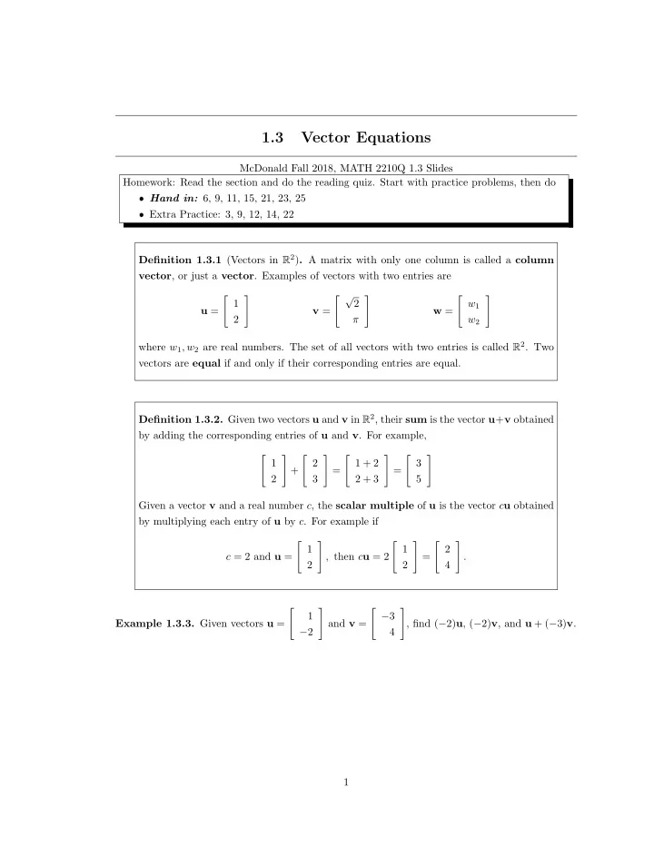
  1. 1.3 Vector Equations McDonald Fall 2018, MATH 2210Q 1.3 Slides Homework: Read the section and do the reading quiz. Start with practice problems, then do ❼ Hand in: 6, 9, 11, 15, 21, 23, 25 ❼ Extra Practice: 3, 9, 12, 14, 22 Definition 1.3.1 (Vectors in R 2 ) . A matrix with only one column is called a column vector , or just a vector . Examples of vectors with two entries are � √ � � � � � 1 2 w 1 u = v = w = 2 π w 2 where w 1 , w 2 are real numbers. The set of all vectors with two entries is called R 2 . Two vectors are equal if and only if their corresponding entries are equal. Definition 1.3.2. Given two vectors u and v in R 2 , their sum is the vector u + v obtained by adding the corresponding entries of u and v . For example, � � � � � � � � 1 2 1 + 2 3 + = = 2 3 2 + 3 5 Given a vector v and a real number c , the scalar multiple of u is the vector c u obtained by multiplying each entry of u by c . For example if � � � � � � 1 1 2 c = 2 and u = , then c u = 2 = . 2 2 4 � � � � 1 − 3 Example 1.3.3. Given vectors u = and v = , find ( − 2) u , ( − 2) v , and u + ( − 3) v . − 2 4 1

  2. � a Observation 1.3.4 (Vectors in R 2 ) . We can identify the column vector � with the b point ( a, b ) in the plain, so we can consider R 2 as the set of all points in the plain. We usually visualize a vector by including an arrow from the origin. � � � � 2 − 6 Example 1.3.5. Let u = and v = . Graph u , v and u + v on the plane. 2 1 Proposition 1.3.6 (Parallelogram Rule) . If u and v in R 2 are represented in the plain, then u + v corresponds to the last vertex of the parallelogram with vertices are u , v and 0 . � � 1 Example 1.3.7. Let u = . Graph u , ( − 2) u , and 3 u . What’s special about c u for any c ? − 1 Observation 1.3.8 (Vectors in R 3 ) . Vectors in R 3 are 3 × 1 matrices. Like above, we can represent them geometrically in three-dimensional coordinate space. For example,   2 a = 3     4 2

  3. Definition 1.3.9 (Vectors in R n ) . If n is a positive integer, R n denotes the collection of ordered n -tuples of n real numbers, usually written as n × 1 column matrices, such as   a 1 a 2     a = , .   . .     a n we we again, sometimes denote ( a 1 , a 2 , . . . , a n ). The zero vector , denoted 0 is the vector whose entries are all zero. We also denote ( − 1) u = − u . Proposition 1.3.10 (Algebraic Properties of R n ) . For u , v , w in R n , and scalars c , d : (i) u + v = v + u (v) c ( u + v ) = c u + c v (ii) ( u + v ) + w = u + ( v + w ) (vi) ( c + d ) u = c u + d u (iii) u + 0 = 0 + u = u (vii) c ( d u ) = ( cd ) u (iv) u + ( − u ) = − u + u = 0 (viii) 1 u = u   a 1 a 2     Remark 1.3.11. Sometimes, for ease of notation, we denote as ( a 1 , a 2 , . . . , a n ). .   .  .    a n Example 1.3.12. Prove properties (i) and (v) of the Algebraic Properties above. 3

  4. Definition 1.3.13 (Linear Combinations) . Given vectors v 1 , v 2 , . . . , v m in R n , and scalars c 1 , c 2 , . . . , c m . The vector c 1 v 1 + c 2 v 2 + · · · + c m v m is called a linear combination of the v 1 , . . . v m with weights c 1 , . . . , c m . � 2 � − 1 � � Example 1.3.14. The figure below shows linear combinations of v 1 = and v 2 = where 1 1 with integer weights. Estimate the linear combinations of v 1 and v 2 that produce u and w .       1 2 7 Example 1.3.15. Let a 1 = − 2  , a 2 = 5  , b = 4  . Is b a linear combination of a 1 and a 2 ?          − 5 6 − 3 4

  5. Remark 1.3.16. In the previous example, the vectors a 1 , a 2 and b became the columns of the augmented matrix that we reduced:   1 2 7 − 2 5 4     − 5 6 − 3 � � For brevity, we will write this matrix, using vectors, as . This suggests the following. a 1 a 2 b Procedure 1.3.17. A vector equation x 1 a 1 + · · · + x n a n = b , has the same solution set as the linear system whose augmented matrix is � � a 1 · · · a n b In particular, b can be represented as a linear combination of a 1 , . . . , a n if and only if there is a solution to the linear system corresponding to this matrix. Definition 1.3.18. If v 1 , . . . , v m are in R n , then the set of all linear combinations of is denoted by Span { v 1 , . . . , v m } and is called the subset of R n spanned by v 1 , . . . , v m . In other words, Span { v 1 , . . . , v m } is the collection of all vectors of the form c 1 v 1 + c 2 v 2 + · · · + c m v m , with c 1 , . . . , c m scalars. � � � � − 1 2 Example 1.3.19. Let v 1 = and v 2 = . Prove that v 1 and v 2 span all of R 2 . 1 1 5

  6. Remark 1.3.20. Actually, for any u and v (which are not multiples) in R 3 , Span { u , v } is a plane! Observation 1.3.21 (Geometric Descriptions of Span { u } and Span { u , v } ) . Let u and v be nonzero vectors in R 3 , with u not a multiple of v . Then Span { v } is the set of points on the line in R 3 through 0 and v , and Span { u , v } is the plane in R 3 containing 0 , u and v , that is, it contains the line in R 3 through u and the line through 0 and v and 0 .     1 5 Example 1.3.22. If a 1 =  , a 2 =  . Is ( − 3 , 8 , 1) in the plane spanned by a 1 and a 2 ? − 2 − 13       3 − 3 6

Download Presentation
Download Policy: The content available on the website is offered to you 'AS IS' for your personal information and use only. It cannot be commercialized, licensed, or distributed on other websites without prior consent from the author. To download a presentation, simply click this link. If you encounter any difficulties during the download process, it's possible that the publisher has removed the file from their server.

Recommend


More recommend