09-12-2019 Outline Introduction to Dynamic Linear Models (DLM) - - - PDF document

09-12-2019 1

Monitoring and data filtering II

Dan Jensen IPH, KU

Outline

Introduction to Dynamic Linear Models (DLM)

• Conceptual introduction
• Difference between the ”Classical methods” and DLM
• A very simple DLM and the Kalman filter
• Break (5 minutes)

Appliction examples using the simple DLM

• Break (10 minutes)

General form of the DLM Appliction examples using the general DLM Concluding remarks and Exercises Estimation

The basics of a DLM

Dynamic

i.e. non-static, adaptive

Forecasted value Observed value Uncertainties TRUE VALUE

The basics of a DLM

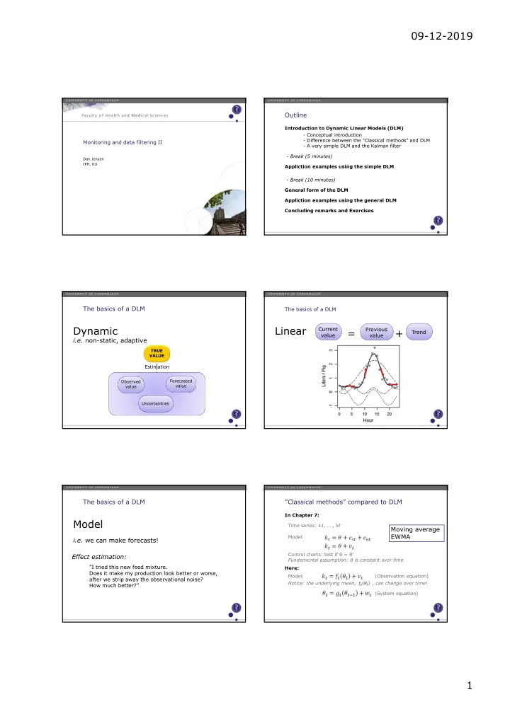
Linear

Current value

=

Previous value

+

Trend

The basics of a DLM

Model

i.e. we can make forecasts!

IF “everything is fine” THEN “things progress as expected” Therefore: IF “things progress UN-expectedly” THEN “Something is wrong!”

Alarm system:

”If I stay the course, how will my production look

• ver the next few years?”

”How will it look if I change to a faster growing breed?”

Decision support:

”I tried this new feed mixture. Does it make my production look better or worse, after we strip away the observational noise? How much better?”

Effect estimation: ”Classical methods” compared to DLM

In Chapter 7: Here: Time series: k1, … , kt Model: Control charts: test if θ = θ’ Fundemental assumption: θ is constant over time Notice: the underlying mean, , can change over time! Model: (Observation equation) (System equation)

Moving average EWMA

09-12-2019 2

First Order Univariate Polynomial DLM

A very simple DLM Updated with each time step!

Adaptive coefficient Forecast error

Updating the (simple) DLM: the Kalman filter

Prior information: 1-step forecast information: Adaptation information Filtered (posterior) information Prior mean Prior variance Forecast Forecast variance Filtered mean Filtered variance

Relation to the EWMA

EWMA: Filtered mean: When and :

Incorporate external information

Incorporate external information: intervention Types of external information:

• 1. Known effect, experienced before

(ex: new breed with a known different performance) → We want the model to adapt to the new known conditions

• 2. Unknown effect

(ex: wave of heat, introduction of new animals in a group) → We want the model to adapt to the new unknown conditions

• 3. Unknown effect we want to measure

(ex: change of feed composition, new veterinary treatments) → We want to measure the effect of a voluntary change

Intervention - 1. Known effect We want the model to adapt to the new known conditions

• Ex. 8.4, p. 88: Productivity in broilers / reference weight 38 days

V=10000 g2 (i.e. SD of 333 g) Until batch 10: Ross 208; m10 = 1883 g, W= 100 g2 From batch 11: Ross 308, Δ » N (μ Δ, W Δ) where μ Δ= 70 and W Δ = 100 Revised prior: (θt’ | Dt’-1) » N(mt’-1 + μ Δ, Rt’), Rt’ = Ct’-1 + Wt’ + W Δ m11 = m10 + 70 = 1883 + 70 = 1953 And R11 = C10 + W11 + W Δ = 1201+ 100 +100 = 1401

Incorporate external information

09-12-2019 3

Incorporate external information

Intervention - 2. Unknown effect We want the model to adapt to the new unknown conditions Ex 1: broiler example with no prior information Δ ~ N (0, 20000) for t = 11 In practice we temporarily apply a larger system variance W

Incorporate external information

Intervention - 2. Unknown effect Productivity in broilers / reference weight Change in production should be modeled as intervention If any prior information is available: use it !

Intervention, prior knowlegde Δ ~ N (70, 100) Intervention, no prior knowlegde Δ ~ N (0, 20000) No intervention

Incorporate external information

Intervention - 3. Estimation of effect Productivity in broilers / reference weight

+ 75 g

Smoothing Retrospective analysis

Intervention, no prior knowlegde Δ ~ N (0, 20000) Smoothed mean

The general Dynamic Linear Model

Definition In a general DLM, observations may be multivariate (i.e. vectors) Let Yt = (y1, … , yn)’ be a vector of key figures observed at time t. Let θt = (θ1, … , θm)’ be a vector of parameters describing the system at time t. General form of the DLM Observation Equation: Yt = F’t θt + νt , νt ~ N(0,Vt) System Equation: θt = Gt θt-1 + ωt, ωt ~ N(0,Wt) Ft is the design matrix: extracts expected observations from θt Gt is the system matrix: describe how θt changes over time DLM combined with Kalman Filter: estimate the underlying state vector θt by its mean vector mt and its variance-covariance matrix Ct. A linear growth model Parameter vector Design matrix Observation equation kt = F’ t θt + νt , νt ~ N(0,Vt) System matrix Covariance matrix System equation θt = Gt θt-1 + ωt, ωt ~ N(0,Wt)

Modeling patterns with a DLM         = 0 1

t

F         =

t t 2 1

θ θ θ         = 1 1 1

t

G         =

t t t

W W W

2 1

09-12-2019 4

Updating the general DLM

Prior information: 1-step forecast information: Adaptation information Filtered (posterior) information Prior mean Prior variance Forecast Forecast variance Adaptive coefficient Forecast error Filtered mean Filtered variance

A linear growth model: example of daily feed intake Specification of the priors Observational variance: V = 90000 (i.e. 300 g standard deviation) Evolution variance: delta = 0.98

Modeling patterns with a DLM         = 100 10000 C         = 25 600 m

A linear trend + a cyclically repeating pattern:

• Section-level water consumption of weaned pigs

Modeling patterns with a DLM

A linear trend + a cyclically repeating pattern:

• Section-level water consumption of weaned pigs
• Parameter estimation

Modeling patterns with a DLM Sine-Cosine transformation of one wave

A linear trend + a cyclically repeating pattern:

• Section-level water consumption of weaned pigs - Parameter estimation

Modeling patterns with a DLM

8x8 matrix

A linear growth model: example of daily feed intake

System matrix Design matrix

Modeling patterns with a DLM

Observation Equation: Yt = F’t θt + νt , νt ~ N(0,Vt) System Equation: θt = Gt θt-1 + ωt, ωt ~ N(0,Wt)

09-12-2019 5

A linear trend + a cyclically repeating pattern:

• Section-level water consumption of weaned pigs

Modeling patterns with a DLM

Red lines: Forecasted values Blue line: expected daily mean value Green rugs: days with medical treatment of the animals

Monitoring Deviations from the model

First of all: use standardized errors: Then: Control chart, with alarm limits Or V-mask (parameters d and Ψ) Applied on the cumulative sum (cusum) of the standardized error: Or: Others, e.g. Bayesian networks, neural networks, etc.

1 1 − =

+ = = 

t t t t t t

c u u C Concluding remarks

Differents Models were presented

• Simple local level model
• DLM in its general form
• Examples

The general form of the model allows us to include patterns (e.g. cyclic patterns for for drinking activity, linear patterns for daily gain) Not necessarily as graphs – automatic alarms Many handles to adjust – be careful! Always combine with your knowledge on animal production Next time: how to define the variance components!