? 0 1 0 0 0 0 0 0 0 - 1 1 1 = ? * 0 2 0 1 1 1 - - PDF document

Filters, Features, Edges

Thursday, Sept 11

Last time

• Cross correlation
• Convolution
• Examples of smoothing filters

– Box filter (averaging) – Gaussian

Convolution

• Convolution:

– Flip the filter in both dimensions (bottom to top, right to left) – Then apply cross-correlation

Notation for convolution

• perator

F H

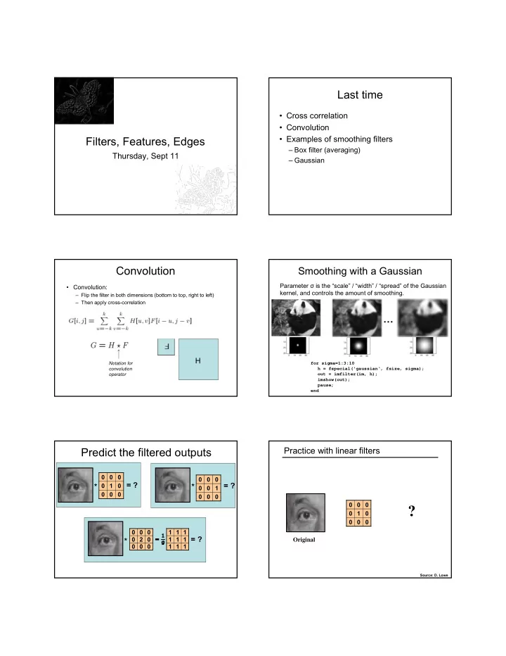
Smoothing with a Gaussian

for sigma=1:3:10 h = fspecial('gaussian‘, fsize, sigma);

• ut = imfilter(im, h);

imshow(out); pause; end

…

Parameter σ is the “scale” / “width” / “spread” of the Gaussian kernel, and controls the amount of smoothing.

Predict the filtered outputs

1

* = ?

1

* = ?

1 1 1 1 1 1 1 1 1 2

• *

= ?

Practice with linear filters

1 Original

?

Source: D. Lowe

Practice with linear filters

1 Original Filtered (no change)

Source: D. Lowe

Practice with linear filters

1 Original

?

Source: D. Lowe

Practice with linear filters

1 Original Shifted left by 1 pixel with correlation

Source: D. Lowe

Practice with linear filters

Original

?

1 1 1 1 1 1 1 1 1

Source: D. Lowe

Practice with linear filters

Original 1 1 1 1 1 1 1 1 1 Blur (with a box filter)

Source: D. Lowe

Practice with linear filters

Original 1 1 1 1 1 1 1 1 1 2

• ?

Source: D. Lowe

Practice with linear filters

Original 1 1 1 1 1 1 1 1 1 2

• Sharpening filter
• Accentuates differences

with local average

Source: D. Lowe

Filtering examples: sharpening Shift invariant linear system

• Shift invariant:

– Operator behaves the same everywhere, i.e. the value of the output depends on the pattern in the image neighborhood, not the position of the neighborhood.

• Linear:

– Superposition: h * (f1 + f2) = (h * f1) + (h * f2) – Scaling: h * (k f) = k (h * f)

Properties of convolution

• Linear & shift invariant
• Commutative:

f * g = g * f

• Associative

(f * g) * h = f * (g * h)

• Identity:

unit impulse e = […, 0, 0, 1, 0, 0, …]. f * e = f

• Differentiation:

Separability

• In some cases, filter is separable, and we can factor into

two steps: – Convolve all rows – Convolve all columns

Separability

• In some cases, filter is separable, and we can factor into

two steps: e.g.,

What is the computational complexity advantage for a separable filter of size k x k, in terms of number of

• perations per output pixel?

f * (g * h) = (f * g) * h g h f

Effect of smoothing filters

5x5

Additive Gaussian noise Salt and pepper noise

Median filter

• No new pixel values

introduced

• Removes spikes: good

for impulse, salt & pepper noise

• Linear?

Median filter

Salt and pepper noise Median filtered

Source: M. Hebert

Plots of a row of the image

Median filter

• Median filter is edge preserving

Filters for features

• Previously, thinking of filtering

as a way to remove or reduce noise

• Now, consider how filters will

allow us to abstract higher-level “features”.

– Map raw pixels to an intermediate representation that will be used for subsequent processing – Goal: reduce amount of data, discard redundancy, preserve what’s useful

Template matching

• Filters as templates:

Note that filters look like the effects they are intended to find --- “matched filters”

• Use normalized cross-correlation score to find a

given pattern (template) in the image.

• Normalization needed to control for relative

brightnesses.

Template matching

Scene Template (mask)

A toy example

Template matching

Template Detected template

Template matching

Detected template Correlation map

Where’s Waldo?

Scene Template

Where’s Waldo?

Detected template Template

Where’s Waldo?

Detected template Correlation map

Template matching

Scene Template

What if the template is not identical to some subimage in the scene?

Template matching

Detected template Template

Match can be meaningful, if scale, orientation, and general appearance is right.

Edge detection

• Goal: map image from 2d array of pixels to a set of

curves or line segments or contours.

• Why?
• Main idea: look for strong gradients, post-process

Figure from J. Shotton et al., PAMI 2007

What can cause an edge?

Depth discontinuity:

• bject boundary

Change in surface

• rientation: shape

Cast shadows Reflectance change: appearance information, texture

Contrast and invariance

Recall : Images as functions

Edges look like steep cliffs

Source: S. Seitz

Derivatives and edges

image intensity function (along horizontal scanline) first derivative edges correspond to extrema of derivative

Source: L. Lazebnik

An edge is a place of rapid change in the image intensity function.

Differentiation and convolution

For 2D function, f(x,y), the partial derivative is: For discrete data, we can approximate using finite differences: To implement above as convolution, what would be the associated filter?

ε ε

ε

) , ( ) , ( lim ) , ( y x f y x f x y x f − + = ∂ ∂

→

1 ) , ( ) , 1 ( ) , ( y x f y x f x y x f − + ≈ ∂ ∂

Partial derivatives of an image

Which shows changes with respect to x?

• 1

1 1

• 1
• r

?

• 1 1

x y x f ∂ ∂ ) , ( y y x f ∂ ∂ ) , (

(showing flipped filters)

Assorted finite difference filters

>> My = fspecial(‘sobel’); >> outim = imfilter(double(im), My); >> imagesc(outim); >> colormap gray;

Image gradient

The gradient of an image: The gradient points in the direction of most rapid change in intensity The gradient direction (orientation of edge normal) is given by: The edge strength is given by the gradient magnitude

Slide credit S. Seitz

Effects of noise

Consider a single row or column of the image

• Plotting intensity as a function of position gives a signal

Where is the edge?

Where is the edge?

Solution: smooth first

Look for peaks in

Derivative theorem of convolution

Differentiation property of convolution.

Derivative of Gaussian filter

[ ]

1 1 − ⊗

[ ]

0.0030 0.0133 0.0219 0.0133 0.0030 0.0133 0.0596 0.0983 0.0596 0.0133 0.0219 0.0983 0.1621 0.0983 0.0219 0.0133 0.0596 0.0983 0.0596 0.0133 0.0030 0.0133 0.0219 0.0133 0.0030

) ( ) ( h g I h g I ⊗ ⊗ = ⊗ ⊗

Why is this preferable?

Derivative of Gaussian filters

x-direction y-direction

Source: L. Lazebnik

Laplacian of Gaussian

Consider

Laplacian of Gaussian

• perator

Where is the edge? Zero-crossings of bottom graph

2D edge detection filters

• is the Laplacian operator:

Laplacian of Gaussian Gaussian derivative of Gaussian

Mask properties

• Smoothing

– Values positive – Sum to 1 constant regions same as input – Amount of smoothing proportional to mask size – Remove “high-frequency” components; “low-pass” filter

• Derivatives

– Opposite signs used to get high response in regions of high contrast – Sum to 0 no response in constant regions – High absolute value at points of high contrast

• Filters act as templates
• Highest response for regions that “look the most like the filter”
• Dot product as correlation

Gradients -> edges

Primary edge detection steps:

• 1. Smoothing: suppress noise
• 2. Edge enhancement: filter for contrast
• 3. Edge localization

Determine which local maxima from filter output are actually edges vs. noise

• Threshold, Thin

Smoothing with a Gaussian

Recall: parameter σ is the “scale” / “width” / “spread” of the Gaussian kernel, and controls the amount of smoothing.

… Effect of σ on derivatives

The apparent structures differ depending on Gaussian’s scale parameter. Larger values: larger scale edges detected Smaller values: finer features detected

σ = 1 pixel σ = 3 pixels

So, what scale to choose?

It depends what we’re looking for. Too fine of a scale…can’t see the forest for the trees. Too coarse of a scale…can’t tell the maple grain from the cherry.

Thresholding

• Choose a threshold value t
• Set any pixels less than t to zero (off)
• Set any pixels greater than or equal to t to one (on)

Original image Gradient magnitude image Thresholding gradient with a lower threshold Thresholding gradient with a higher threshold

Canny edge detector

• Filter image with derivative of Gaussian
• Find magnitude and orientation of gradient
• Non-maximum suppression:

– Thin multi-pixel wide “ridges” down to single pixel width

• Linking and thresholding (hysteresis):

– Define two thresholds: low and high – Use the high threshold to start edge curves and the low threshold to continue them

• MATLAB: edge(image, ‘canny’);
• >>help edge

Source: D. Lowe, L. Fei-Fei

The Canny edge detector

• riginal image (Lena)

The Canny edge detector

norm of the gradient

The Canny edge detector

thresholding

The Canny edge detector

thresholding How to turn these thick regions of the gradient into curves?

Non-maximum suppression

Check if pixel is local maximum along gradient direction, select single max across width of the edge

• requires checking interpolated pixels p and r

The Canny edge detector

thinning (non-maximum suppression)

Problem: pixels along this edge didn’t survive the thresholding

Hysteresis thresholding

• Check that maximum value of gradient value

is sufficiently large – drop-outs? use hysteresis

• use a high threshold to start edge curves and a

low threshold to continue them.

Source: S. Seitz

Hysteresis thresholding

• riginal image

high threshold (strong edges) low threshold (weak edges) hysteresis threshold

Source: L. Fei-Fei

Object boundaries vs. edges

Background Texture Shadows

Edge detection is just the beginning…

Berkeley segmentation database:

http://www.eecs.berkeley.edu/Research/Projects/CS/vision/grouping/segbench/

image human segmentation gradient magnitude

Source: L. Lazebnik

[D. Martin et al. PAMI 2004]

Human-marked segment boundaries

Possible to learn from humans which combination of features is most indicative

• f a “good”

contour?

Feature profiles (oriented energy, brightness, color, and texture gradients) along the patch’s horizontal diameter

[D. Martin et al. PAMI 2004]

What features are responsible for perceived edges?

[D. Martin et al. PAMI 2004]

Summary

• Filters allow local image neighborhood to influence our

description and features

– Smoothing to reduce noise – Derivatives to locate contrast, gradient

• Filters have highest response on neighborhoods that

“look like” it; can be thought of as template matching.

• Convolution properties will influence the efficiency with

which we can process images.

– Associative – Filter separability

• Edge detection processes the image gradient to find

curves, or chains of edgels.

Next

• Tues 9/16 binary images
• Reminder: Pset 1 due Sept 18.

Seam Carving

• Energy function:
• Want to remove or insert seams where they won’t be

very noticeable

• Choose seam based on minimum total energy path

across image.