Zeroes When working with n-gram models, zero probabilities can be - - PDF document

1

Smoothing and Backoff Zeroes

• When working with n-gram models, zero

probabilities can be real show-stoppers

• Examples:

– Zero probabilities are a problem

• p(w1 w2 w3...wn) ≈ p(w1) p(w2|w1) p(w3|w2)...p(wn|wn-1) bigram

model

• one zero and the whole product is zero

– Zero frequencies are a problem

• p(wn|wn-1) = C(wn-1wn)/C(wn-1)

relative frequency

• word doesn’t exist in dataset and we’re dividing by

zero

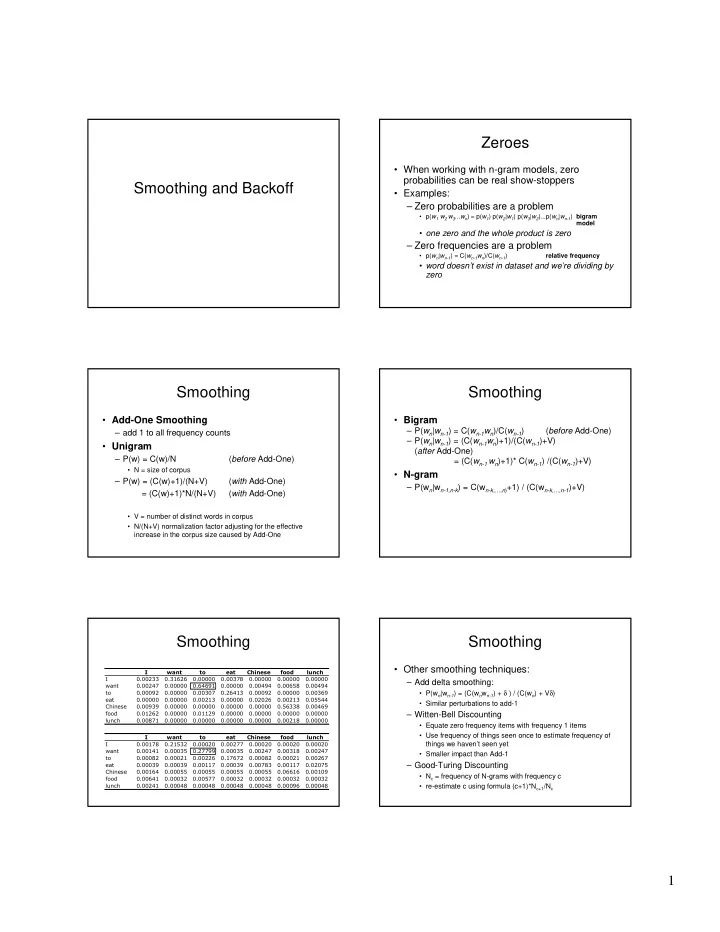
Smoothing

• Add-One Smoothing

– add 1 to all frequency counts

• Unigram

– P(w) = C(w)/N (before Add-One)

• N = size of corpus

– P(w) = (C(w)+1)/(N+V) (with Add-One) = (C(w)+1)*N/(N+V) (with Add-One)

• V = number of distinct words in corpus
• N/(N+V) normalization factor adjusting for the effective

increase in the corpus size caused by Add-One

Smoothing

• Bigram

– P(wn|wn-1) = C(wn-1wn)/C(wn-1) (before Add-One) – P(wn|wn-1) = (C(wn-1wn)+1)/(C(wn-1)+V) (after Add-One) = (C(wn-1 wn)+1)* C(wn-1) /(C(wn-1)+V)

• N-gram

– P(wn|wn-1,n-k) = C(wn-k,…,n)+1) / (C(wn-k,…,n-1)+V)

Smoothing

• Smoothing
• Other smoothing techniques:

– Add delta smoothing:

• P(wn|wn-1) = (C(wnwn-1) + δ ) / (C(wn) + Vδ)
• Similar perturbations to add-1

– Witten-Bell Discounting

• Equate zero frequency items with frequency 1 items
• Use frequency of things seen once to estimate frequency of

things we haven’t seen yet

• Smaller impact than Add-1

– Good-Turing Discounting

• Nc = frequency of N-grams with frequency c
• re-estimate c using formula (c+1)*Nc+1/Nc

2

Good Turing

• Basic concept: probability of events with

counts > 1 is decreased (discounted) and probability of events with counts = 0 is increased

• Essentially we save some of the

probability mass from seen events and make it available to unseen events

• Allows us to estimate the probability of

zero-count events

Good Turing

• Good Turing gives a smoothed count c* based
• n the set of Nc for all c:

Nc+1 c* = (c+1) -------- Nc

• Example: revised count for bigrams that never
• ccurred (c0) = c1 *

# of bigrams that occurred once

• # bigrams that never occurred

Good Turing

• Bigram counts from 22 million AP

newswire (Church & Gale 1991):

Good Turing

• Good Turing
• How do we get this number?

– For bigrams, total vocabulary = (unigram vocabulary)2 – Thus, 74,671,100,000 = V2 – (seen bigrams)

Applying Good Turing

• So we have these new counts
• What do we do with them?

– Apply them to our probability calculations!

3

Uniform Good Turing

• Uniform application:

– (Examples use bigrams) – To calculate the probability of any bigram, we use:

• P ( wn|wn-1) = C(wn-1 wn) / C(wn-1)

– Apply the revised c* values to our probabilities – Thus revised c* substituted for C(wn-1 wn)

• P ( wn|wn-1) = cn

* / C(wn-1)

Uniform Good Turing

– Thus, if C(she drove) = 6, then c* = 5.19 – If C(she)=192, then

• Revised P(drove|she) = 5.19/192 = .02703

(revised from .03125)

Uniform Good Turing

– What’s the probability of some unknown bigram? – For example, if C(gave she) = 0, then c*=.000027 – If C(gave) = 154, then

• P(gave she) = .000027/154 = .000000175

Applying Good Turing

• Is a uniform application of Good Turing the

right thing to do?

• Can we assume that

C(any unseen bigram) = C(any other unseen)?

• Church and Gale 91 show a method for

calculating the P(unseen bigram) from the P(unseen) and P(bigram)

– Works only if the unigrams for both words exist

Unigram-sensitive Good Turing

• How it works (for unseen bigrams):

– Calculate the joint probability P(wn)P(wn+1) – Group bigrams into bins based on similar joint probability scores

• Predetermined set of ranges and thresholds

– Do Good Turing estimation on each of the bins

• In other words, smooth (normalize the probability

mass) across each of the bins separately

Good Turing

• Katz 1987 showed that Good Turing for large

counts reliable

• Based on his work, smoothing in practice not

applied to large c’s.

• Proposed some threshold k (he recommended

5) where c* = c for c > k.

• Still smooth for c <= k
• May also want to treat n-grams with low counts

(especially 1) as zeroes.

4

Backoff

• Assumes additional sources of knowledge:

– If we don’t have a value for a particular trigram probability, P(wn|wn-1wn-2) – We can estimate the probability by using the bigram probability: P(wn|wn-1) – If we don’t have a value for this bigram, we can look at the unigram probability: P(wn). – If we do have the trigram probability P(wn|wn-1wn-2), we use it. – We only “backoff” to the lower-order if no evidence for the higher order.

Backoff

• Preference rule:
• P^(wn|wn-2wn-1) =

1. P(wn |wn-2 wn-1) if C(wn-2wn-1 wn ) ≠ 0, else 2. α1P(wn|wn-1 ) if C(wn-1 wn ) ≠ 0, else 3. α2P(wn)

• α values are used to normalize probability

mass so that it still sums to 1, and to “smooth” the lower order probabilities that are used

• See J&M § 6.4 for details of how to calculate α

values (and M&S § 6.3.2 for additional discussion)

Interpolation

• Rather than choosing between different models

(trigram, bigram, unigram), as in backoff

• Interpolate the models when computing a

trigram

• Proposed first by Jelinek and Mercer (1980)
• P^(wn |wn-2 wn-1) =

λ1P(wn |wn-2 wn-1) + λ2P(wn |wn-2 ) + λ3P(wn )

• Where Σ λi = 1

i

X X

Interpolation

• Generally, here’s what’s done:

– Split data into training, held-out, and test – Train model on training set – Use held-out to test different λ values and pick the

• nes that works best

– Test the model on the test data

• Held-out: used to smooth model, and to ensure

model is not over-training (over-specifying)

• Cardinal sin: testing on training data