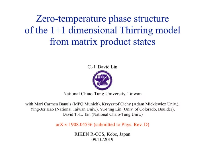
Zero-temperature phase structure of the 1+1 dimensional Thirring - PowerPoint PPT Presentation

Zero-temperature phase structure of the 1+1 dimensional Thirring model from matrix product states C.-J. David Lin National Chiao-Tung University, Taiwan with Mari Carmen Banuls (MPQ Munich), Krzysztof Cichy (Adam Mickiewicz Univ.), Ying-Jer Kao (National Taiwan Univ.), Yu-Ping Lin (Univ. of Colorado, Boulder), David T.-L. Tan (National Chaio-Tung Univ.) arXiv:1908.04536 (submitted to Phys. Rev. D) RIKEN R-CCS, Kobe, Japan 09/10/2019

Outline • Preliminaries: motivation and introduction • Lattice formulation and the MPS • Simulations and numerical results: 
 Phase structure of the Thirring model • Remarks and outlook (spectrum, real-time dynamics)

Preliminaries

Logic flow Hamiltonian formalism for QFT Quantum spin model MPS & variational method for obtaining the ground state Compute correlators and excited state spectrum

Motivation • New formulation for lattice field theory • No sign problem • Real-time dynamics • Future quantum computers? In this talk: BKT phase transition

The 1+1 dimensional Thirring model � ¯ � � ¯ � g Z h �i S Th [ , ¯ i � µ @ µ � m ¯ ¯ d 2 x � µ ] = � µ 2 Conformality of the massless theory Duality with the sine-Gordon theory


 
 Bosonisation and duality • Basic ingredients from free field theories 
 � n � ( µ | x i − x j | ) κ i κ j / 2 π , where � e i κ i φ ( x ) � bare = ( Λ /µ ) − κ 2 i / 4 π � e i κ i φ ( x ) � � � e i κ i φ ( x ) = ren . i =1 i<j ren . And similar power law for ¯ ψψ correlators. Works in the zero-charge sector • The dictionary (zero total fermion number) � µ $ 1 � ¯ � ψψ − g ¯ � � 2 � ψ , ¯ ψ i γ µ ∂ µ ψ − m 0 ¯ ¯ 2 ⇡ ✏ µ ν @ ν � , d 2 x � � = S Th ψ ψγ µ ψ 2 $ Λ ¯ ⇡ cos � , field redifinition, anomaly 4 ⇡ t = 1 + g ⇡ . S SG [ φ ] = 1 � 1 � � d 2 x 2 ∂ µ φ ( x ) ∂ µ φ ( x ) + α 0 cos ( φ ( x )) ↵ 0 t = m 0 Λ t . ⇡ m 0 = m ( µ/ Λ ) g/ ( g + π ) , Coleman: Unstable vacuum at g ∼ − π / 2 ↵ 0 = ↵ ( µ/ Λ ) � t/ 4 π .

Dualities and phase structure Thirring sine-Gordon XY 4 π 2 T g − π K − π t Picture from: K. Huang and J. Polonyi, 1991 The K-T phase transition at T ∼ K π / 2 in the XY model. g ⇠ � π / 2, Coleman’s instability point The phase boundary at t ∼ 8 π in the sine-Gordon theory. The cosine term becomes relevant or irrelevant. Thirring sine-Gordon 1 ¯ � µ 2 ⇡ ✏ µ ν @ ν � Λ ¯ ⇡ cos �

RG flows of the Thirring model Perturbative expansion in mass β g ⌘ µ dg ⇣ m ⌘ 2 dµ = � 64 π , Λ 256 π 3  � 2( g + π 2 ) β m ⌘ µdm ⇣ m ⌘ 2 � dµ = m � ( g + π ) 2 g + π Λ

Lattice formulation and the MPS


 
 Operator formalism and the Hamiltonian Operator formaliam of the Thirring model Hamiltonian 
 • C.R. Hagen, 1967 " # ◆ − 1 � ¯ � ¯ ψψ + g � 2 � g ✓ 1 + 2 g Z � 2 � i ¯ ψγ 1 ∂ 1 ψ + m 0 ¯ ψγ 0 ψ ψγ 1 ψ H Th = dx 4 4 π Staggering, J-W transformation ( ): j ± iS y S ± • j = S x j J. Kogut and L. Susskind, 1975; A. Luther, 1976 N − 2 N − 1 N − 1  � 1 ✓ n + 1 ◆ ✓ n + 1 ◆ ✓ n +1 + 1 ◆ � ¯ X X ( � 1) n X S + n +1 + S + S z S z S z � � H XXZ = ν ( g ) n S − n +1 S − + a ˜ m 0 + ∆ ( g ) n 2 2 2 2 n n n 2 γ m 0 = m 0 ν ( g ) , ∆ ( g ) = cos ( γ ) , with γ = π � g ν ( g ) = π sin( γ ) , ˜ 2 projected to a sector of total spin ! 2 N − 1 H (penalty) ¯ = ¯ X S z H XXZ + λ n � S target XXZ JW-trans of the total fermion number, n =0 Bosonise to topological index in the SG theory.

Issue of large Hilbert space & DMRG/MPS S. White, 1992; M.B. Hasting, 2004; F. Verstraeten and I. Cirac, 2006; … | i 2 dim( H ) = O ( d n ) . big: For a spin system of size n and local dimension d , the d d X X | ψ i = c j 1 ,...,j n | j 1 , . . . , j n i = c j 1 ,...,j n | j 1 i ⌦ · · · ⌦ | j n i j 1 ,...,j n =1 j 1 ,...,j n =1 Entanglement-based truncation of the Hilbert space (Area law of the entanglement entropy)

Matrix product states in a nutshell | i 2 d d X X | ψ i = c j 1 ,...,j n | j 1 , . . . , j n i = c j 1 ,...,j n | j 1 i ⌦ · · · ⌦ | j n i j 1 ,...,j n =1 j 1 ,...,j n =1 bers. While Entanglement-based O ( d n ) man argument for choosing D many real (DMRG via MPS) by O ( ndD 2 ) Bond dim xponential in : so . D A (1) α ; j 1 A (2) β , γ ; i 2 . . . A ( n ) ω ; j n = A (1) j 1 A (2) j 2 . . . A ( n ) X c j 1 ,...,j n = j n , α ,..., ω =1

Matrix Product Operator ⇣ ⌘ b l − 1 X ˆ A i ˆ ˆ B i +1 + ˆ B i ˆ O = A i +1 i ˆ = ˆ A ⊗ ˆ B ⊗ 1 ⊗ · · · ⊗ 1 b l − 1 + 1 ⊗ ˆ A ⊗ ˆ B ⊗ 1 ⊗ · · · ⊗ 1 + · · · + ˆ B ⊗ ˆ A ⊗ 1 ⊗ · · · ⊗ 1 + 1 ⊗ ˆ B ⊗ ˆ A ⊗ 1 ⊗ · · · ⊗ 1 + · · · σ L − 1 , σ ′ M σ 1 , σ ′ 1 ,b 1 M σ 2 , σ ′ b 1 ,b 2 M σ 3 , σ ′ b L − 3 ,b L − 1 M σ L , σ ′ ˆ � L − 1 O = b 2 ,b 3 . . . M L 1 2 3 b L − 1 , 1 b 1 ,...,b L − 1 σ 1 σ σ L σ 1 σ σ L b 1 b - 1 b b L -1 σ ´ 1 σ ´ σ ´ L σ ´ 1 σ ´ σ ´ L matrix elements It is simple to compute local operator matrix elements with canonical states.


 
 
 
 
 
 
 Simulation details for the phase structure Matrix product operator for the Hamiltonian (bulk) 
 • 2 S − 2 λ S z ∆ S z β n S z + α 1 2 × 2 2 S + − 1 1 2 × 2 − 1 0 1 0 0 0 0 0 S − B C S + 0 0 0 0 0 B C W [ n ] = B C S z 0 0 0 1 0 B C B C S z 0 0 0 0 0 @ A 0 0 0 0 0 1 2 × 2 ! 4 + S 2 1 + ∆ β n = ∆ + ( − 1) n ˜ target m 0 a − 2 λ S target , α = λ N 4 Simulation parameters • Twenty values of , ranging from -0.9 to 1.0 ∆ ( g ) Fourteen values of , ranging from 0 to 0.4 m 0 a ˜ Bond dimension D = 50 , 100 , 200 , 300 , 400 , 500 , 600 System size N = 400 , 600 , 800 , 1000

Practice of MPS for DMRG a -1 a σ L σ ´ a -1 ´ a ´ One step in a sweep of finite-size DMRG

Simulations and numerical results

6 Convergence of DMRG Start from random tensors at D=50, then go up in D • ⇠ DMRG converges fast at and ∆ ( g ) > • m 0 a 6 = 0 ˜ ⇠ � 0 . 7

Entanglement entropy Calabrese-Cardy scaling and the central charge  N ⌘� S N ( n ) = c ⇣ π n 6 ln π sin + k , N 1 . 4 1 . 6 1 . 3 1 . 2 1 . 4 S N ( n ) S N ( n ) 1 . 1 1 . 2 1 . 0 D = 100 D = 100 1 . 0 0 . 9 D = 200 D = 200 0 . 8 D = 400 D = 400 0 . 8 ∆ ( g ) = − 0 . 88 , ˜ m 0 a = 0 . 0 ∆ ( g ) = 0 . 0 , ˜ m 0 a = 0 . 0 D = 600 D = 600 0 . 7 0 200 400 600 800 1000 0 200 400 600 800 1000 site n site n ∼ − Calabrese-Cardy scaling observed at all values of for m 0 a = 0 d ∆ ( g ) = 0 ˜

Entanglement entropy Calabrese-Cardy scaling and the central charge  N ⌘� S N ( n ) = c ⇣ π n 6 ln π sin + k , N 0 . 505 1 . 0 0 . 500 1 . 6 0 . 495 0 . 9 1 . 4 0 . 490 S N ( n ) S N ( n ) S N ( n ) 1 . 2 0 . 485 0 . 8 1 . 0 0 . 480 D = 100 D = 100 D = 100 0 . 7 0 . 475 D = 200 D = 200 D = 200 0 . 8 D = 400 D = 400 D = 400 0 . 470 ∆ ( g ) = − 0 . 88 , ˜ m 0 a = 0 . 2 ∆ ( g ) = − 0 . 7 , ˜ m 0 a = 0 . 2 ∆ ( g ) = 0 . 0 , ˜ m 0 a = 0 . 2 D = 600 D = 600 D = 600 0 . 6 0 . 6 0 . 465 0 200 400 600 800 1000 0 200 400 600 800 1000 0 200 400 600 800 1000 site n site n site n ⇠ � Calabrese-Cardy scaling observed at for m 0 a 6 = 0 ˜ ∆ ( g ) < ⇠ � 0 . 7

Entanglement entropy Calabrese-Cardy scaling and the central charge  N ⌘� S N ( n ) = c ⇣ π n 6 ln π sin + k , N 1 . 6 1 . 4 S N ( n ) 1 . 2 1 . 0 D = 100 D = 200 0 . 8 D = 400 ∆ ( g ) = − 0 . 88 , ˜ m 0 a = 0 . 2 D = 600 0 . 6 0 . 2 0 . 4 0 . 6 0 . 8 1 . 0 1 � N π sin( π n � 6 ln N ) Central charge is unity in the critical phase

Density-density correlators 1 S z ( n ) S z ( n + x ) � 1 JW trans C zz ( x ) = h ¯ ψψ ( x 0 + x ) ¯ X X X ψψ ( x 0 ) i conn � � � � � � ! S z ( n ) S z ( n + 1) N x N 0 n n n try fitting to zz ( x ) = β x α and C pow C pow − exp ( x ) = Bx η A x zz 1.1 pow fit α -1 C zz ma=0.005 fitted values of A pow-exp fit η C zz ma=0.02 ma=0.08 1.05 -1.5 ma=0.3 1 -2 the parameter α and η fo rs: N = 1000, ˜ m 0 a = 0 . 02. 0.95 -2.5 0.9 -3 0.85 -3.5 -4 0.8 -0.8 -0.6 -0.4 -0.2 0 0.2 0.4 0.6 0.8 1 -1 -0.9 -0.8 -0.7 -0.6 -0.5 -0.4 -0.3 -0.2 -0.1 0 0.1 ∆ (g) ∆ (g) Evidence for a critical phase

Soliton correlators S. Mandelstam, 1975; E. Witten, 1978 ↵ ( x ) ↵ ( y ) = ⌥ i | 2 ⇡ ( x � y ) | − 1 | cµ ( x � y ) | − � 2 g 2 / (2 ⇡ ) 3 † Z y ⇢ � � ( ⇠ ) ⌥ 1 α = ± d ⇠ ˙ � 2 ⇡ i � − 1 2 i � [ � ( y ) � � ( x )] + O ( x � y ) 2 ⇥ : exp : x (35) Vertex operators Soliton operators connecting vortex and anti-vortex Power-law in the critical phase Power-law Exponential-law in the gapped phase Jordan-Wigner m e i ⇡ P n − 1 j = m +1 S z S + j S − transformation n