Zernike Polynomials Fitting irregular and non-rotationally - PDF document

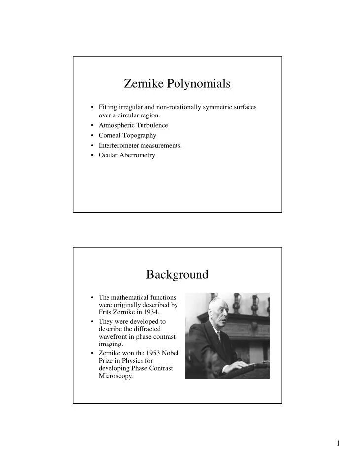
Zernike Polynomials • Fitting irregular and non-rotationally symmetric surfaces over a circular region. • Atmospheric Turbulence. • Corneal Topography • Interferometer measurements. • Ocular Aberrometry Background • The mathematical functions were originally described by Frits Zernike in 1934. • They were developed to describe the diffracted wavefront in phase contrast imaging. • Zernike won the 1953 Nobel Prize in Physics for developing Phase Contrast Microscopy. 1

Phase Contrast Microscopy Transparent specimens leave the amplitude of the illumination virtually unchanged, but introduces a change in phase. Applications • Typically used to fit a wavefront or surface sag over a circular aperture. • Astronomy - fitting the wavefront entering a telescope that has been distorted by atmospheric turbulence. • Diffraction Theory - fitting the wavefront in the exit pupil of a system and using Fourier transform properties to determine the Point Spread Function. Source: http://salzgeber.at/astro/moon/seeing.html 2

Applications • Ophthalmic Optics - fitting corneal topography and ocular wavefront data. • Optical Testing - fitting reflected and transmitted wavefront data measured interferometically. Surface Fitting • Reoccurring Theme: Fitting a complex, non-rotationally symmetric surfaces (phase fronts) over a circular domain. • Possible goals of fitting a surface: – Exact fit to measured data points? – Minimize “Error” between fit and data points? – Extract Features from the data? 3

1D Curve Fitting 25 20 15 10 5 0 -0.1 0.1 0.3 0.5 0.7 0.9 1.1 1.3 1.5 Low-order Polynomial Fit 25 y = 9.9146x + 2.3839 2 = 0.9383 R 20 15 10 5 0 -0.1 0.1 0.3 0.5 0.7 0.9 1.1 1.3 1.5 In this case, the error is the vertical distance between the line and the data point. The sum of the squares of the error is minimized. 4

High-order Polynomial Fit 1800 25 1600 1400 20 1200 1000 15 800 600 10 400 200 5 0 -0.1 0.1 0.3 0.5 0.7 0.9 1.1 1.3 1.5 -200 0 -0.1 -400 0.1 0.3 0.5 0.7 0.9 1.1 1.3 1.5 y = a 0 + a 1 x + a 2 x 2 + … a 16 x 16 Cubic Splines 25 20 15 10 5 0 -0.1 0.1 0.3 0.5 0.7 0.9 1.1 1.3 1.5 Piecewise definition of the function. 5

Fitting Issues • Know your data. Too many terms in the fit can be numerically unstable and/or fit noise in the data. Too few terms may miss real trends in the surface. • Typically want “nice” properties for the fitting function such as smooth surfaces with continuous derivatives. For example, cubic splines have continuous first and second derivatives. • Typically want to represent many data points with just a few terms of a fit. This gives compression of the data, but leaves some residual error. For example, the line fit represents 16 data points with two numbers: a slope and an intercept. Why Zernikes? • Zernike polynomials have nice mathematical properties. – They are orthogonal over the continuous unit circle. – All their derivatives are continuous. – They efficiently represent common errors (e.g. coma, spherical aberration) seen in optics. – They form a complete set, meaning that they can represent arbitrarily complex continuous surfaces given enough terms. 6

Orthogonal Functions • Orthogonal functions are sets of surfaces which have some nice mathematical properties for surface fitting. • These functions satisfy the property = ⎧ C i j ∫∫ = j ⎨ V ( x , y ) V ( x , y ) dxdy i j ⎩ 0 Otherwise A where C j is a constant for a given j Orthogonality and Expansion Coefficients ∑ = W ( x , y ) a V ( x , y ) Linear Expansion i i i ∑ = W ( x , y ) V ( x , y ) a V ( x , y ) V ( x , y ) j i i j i ∑ ∫∫ ∫∫ = W ( x , y ) V ( x , y ) dxdy a V ( x , y ) V ( x , y ) dxdy j i i j i A A 1 ∫∫ = a W ( x , y ) V ( x , y ) dxdy j j C j A 7

Orthogonality - 1D Example Consider the integral π 2 ( ) ( ) ∫ sin mx cos m ' x dx where m and m' are integers 0 π 2 1 [ ] ( ) ( ) ∫ = + + − sin m m ' x sin m m ' x dx 2 0 ( ) ( ) = π + − x 2 ⎡ ⎤ 1 cos m m ' x cos m m ' x = − + ⎢ ⎥ + − ⎣ ⎦ 2 m m ' m m ' = x 0 = 0 Orthogonality - 1D Example Two sine terms π 2 ( ) ( ) ∫ sin mx sin m ' x dx where m and m' are integers 0 π 2 1 [ ] ( ) ( ) ∫ = − + − − cos m m ' x cos m m ' x dx 2 0 ( ) ( ) = π + − x 2 ⎡ ⎤ 1 sin m m ' x sin m m ' x = − − ⎢ ⎥ + − ⎣ ⎦ 2 m m ' m m ' = x 0 = if m ≠ m’ !!! 0 8

Orthogonality - 1D Example Two sine terms with m = m’ π 2 ( ) ( ) ∫ sin mx sin m ' x dx where m and m' are integers 0 π 2 ( ) ∫ = 2 sin mx dx 0 ( ) = π x 2 ⎡ ⎤ x sin 2 mx = − ⎢ ⎥ ⎣ ⎦ 2 4 m = x 0 = π Similar arguments for two cosine terms Orthogonality - 1D Example From the previous arguments, we can define ⎧ ⎛ ⎞ j ⎜ ⎟ cos x ⎪ ⎪ j even ⎝ ⎠ 2 = ⎨ V j ⎛ + ⎞ j 1 j odd ⎪ ⎜ ⎟ sin x ⎪ ⎝ ⎠ ⎩ 2 Note that when j = 0, V 0 = 1 and π π 2 2 = ∫ ( ) ( ) ∫ = π V x V x dx dx 2 0 0 0 0 so the constant C j = 2 π for j = 0, and C j = π for all other values of j. 9

Orthogonality - 1D Example The functions satisfy the orthogonality condition over [0, 2 π ] ( ) π + δ π = ⎧ 2 1 i j ( ) ( ) ∫ = i 0 ⎨ V x V x dx i j ⎩ 0 Otherwise 0 where δ is the Kronecker delta function defined as = ⎧ 1 i j δ = ⎨ ij ⎩ 0 Otherwise Fit to W(x) = x j a j 7 π 0 6 1 -2 5 2 0 3 -1 4 W(x) 1 term 4 0 3 3 terms 11 terms 5 -0.6666 2 6 0 1 7 -0.5 0 0 1 2 3 4 5 6 7 8 0 -1 9 -0.4 10 0 10

Extension to Two Dimensions In many cases, wavefronts take on a complex shape defined over a circular region and we wish to fit this surface to a series of simpler components. Wavefront Fitting -0.003 x = + 0.002 x + 0.001 x 11

Unit Circle y Divide the real radial coordinate by the maximum radius to get a normalized coordinate ρ ρ θ x 1 Orthogonal Functions on the Unit Circle • Taylor polynomials (i.e. 1, x, y, x 2 , xy, y 2 ,….) are not orthogonal on the unit circle. π = ⎧ 2 1 C i j ∫∫ ρ θ ρ θ ρ ρ θ = j ⎨ V ( , ) V ( , ) d d i j ⎩ 0 Otherwise 0 0 where C j is a constant for a given j Many solutions, but let’s try something with the form ( ) ( ) ρ θ = ρ Θ θ V ( , ) R i i i 12

Orthogonal Functions on the Unit Circle • The orthogonality condition separates into the product of two 1D integrals ⎡ ⎤ ⎡ π ⎤ = ⎧ 1 2 C i j ∫ ∫ ρ ρ ρ ρ Θ θ Θ θ θ = j ⎨ ⎢ R ( ) R ( ) d ⎥ ⎢ ( ) ( ) d ⎥ i j i j ⎩ 0 Otherwise ⎣ ⎦ ⎣ ⎦ 0 0 This has extra ρ in it, so This looks like the 1D Example, so sin(m θ ) and cos(m θ ) a possibility we need different functions ANSI Standard Zernikes ⎧ ρ θ ≥ ⎪ m m N R ( ) cos m ; for m 0 ρ θ = m ⎨ n n Z ( , ) n ⎪ − ρ θ < m m ⎩ N R ( ) sin m ; for m 0 n n Azimuthal Double Index Component n is radial order Radial m is azimuthal Component frequency Normalization ANSI Z80.28-2004 Methods for Reporting Optical Aberrations of Eyes. 13

ANSI Standard Zernikes − − − ( n m ) / 2 s ( 1 ) ( n s )! ∑ ρ = ρ − m n 2 s R ( ) [ ] [ ] n + − − − s ! 0 . 5 ( n m ) s ! 0 . 5 ( n m ) s ! = s 0 only depends Constant that depends Powers of ρ on |m| (i.e. same on n and m for both sine & cosine terms The Radial polynomials satisfy the orthogonality equation δ 1 ∫ ρ ρ ρ ρ = m m nn ' R ( ) R ( ) d + n n ' 2 n 2 0 ANSI Standard Zernikes + 2 n 2 = m N + δ n 1 m 0 constant that depends on n & m 14

Orthogonality π = = ⎧ 2 1 C for n n' ; m m' ∫∫ ρ θ ρ θ ρ ρ θ = m ' m n, m ⎨ Z ( , ) Z ( , ) d d n ' n ⎩ 0 Otherwise 0 0 ( ) ( ) π θ θ ⎧ ⎫ ⎧ ⎫ 2 cos m ' cos m ∫ θ m ' m ⎨ ⎬ ⎨ ⎬ N N d ( ) ( ) − θ − θ n ' n ⎩ sin m ' ⎭ ⎩ sin m ⎭ 0 = = ⎧ 1 C for n n' ; m m' ∫ × ρ ρ ρ ρ = m ' m n, m ⎨ R ( ) R ( ) d n ' n ⎩ 0 Otherwise 0 Orthogonality = = δ ⎧ ⎡ ⎤ C for n n' ; m m' [ ] ( ) δ + δ π = m ' m n, m n ' n ⎨ N N 1 ⎢ ⎥ n ' n m ' m m 0 + ⎣ ⎦ ⎩ 0 Otherwise 2 n 2 This equals zero This equals zero So this portion is unless m=m’ unless n=n’ satisfied What happens when n=n’ and m=m’? 15

Orthogonality When n=n’ and m=m’ ( ) ( ⎡ ⎤ [ ] 1 ) 2 + δ π = m N 1 C ⎢ ⎥ n m 0 + n, m ⎣ ⎦ 2 n 2 ⎡ ⎤ + ⎡ ⎤ 2n 2 [ ] 1 ( ) + δ π = ⎢ ⎥ 1 C ⎢ ⎥ + δ + m 0 n , m ⎣ ⎦ ⎣ 1 ⎦ 2 n 2 m0 = π C n , m Orthogonality π 2 1 ∫∫ ρ θ ρ θ ρ ρ θ = πδ δ m ' m Z ( , ) Z ( , ) d d n ' n n ' n m ' m 0 0 16