( ) ( | z ) P ( z ) P Y P Y z 3 Inference - - PDF document

1

1

CS 331: Artificial Intelligence Fundamentals of Probability III

Thanks to Andrew Moore for some course material

2

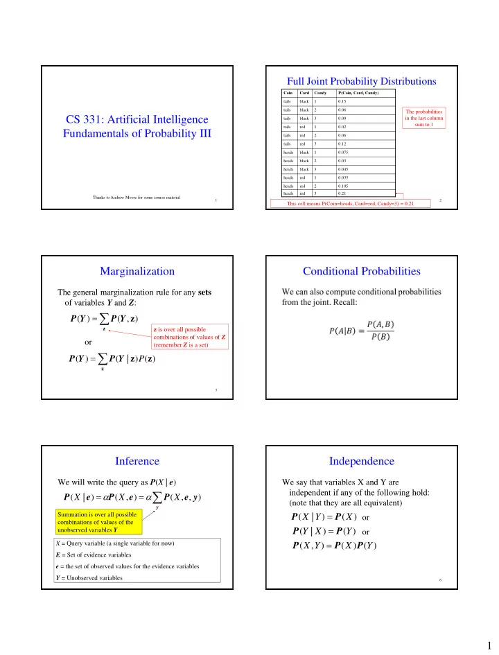
Full Joint Probability Distributions

Coin Card Candy P(Coin, Card, Candy) tails black 1 0.15 tails black 2 0.06 tails black 3 0.09 tails red 1 0.02 tails red 2 0.06 tails red 3 0.12 heads black 1 0.075 heads black 2 0.03 heads black 3 0.045 heads red 1 0.035 heads red 2 0.105 heads red 3 0.21

This cell means P(Coin=heads, Card=red, Candy=3) = 0.21 The probabilities in the last column sum to 1

3

Marginalization

The general marginalization rule for any sets

• f variables Y and Z:





z

z) , ( ) ( Y P Y P





z

z z ) ( ) | ( ) ( P Y P Y P

• r

z is over all possible combinations of values of Z (remember Z is a set)

Conditional Probabilities Inference

We will write the query as P(X | e)



 

y

y e P e P e P ) , , ( ) , ( ) | ( X X X  

X = Query variable (a single variable for now) E = Set of evidence variables e = the set of observed values for the evidence variables Y = Unobserved variables Summation is over all possible combinations of values of the unobserved variables Y

6

Independence

We say that variables X and Y are independent if any of the following hold: (note that they are all equivalent)

) ( ) | ( X Y X P P  ) ( ) | ( Y X Y P P  ) ( ) ( ) , ( Y X Y X P P P 

• r
• r

2

7

Bayes’ Rule

The product rule can be written in two ways: P(A, B) = P(A | B)P(B) P(A, B) = P(B | A)P(A) You can combine the equations above to get: ) ( ) ( ) | ( ) | ( A P B P B A P A B P 

8

Bayes’ Rule

) ( ) ( ) | ( ) | ( B A A B B A P P P P 

More generally, the following is known as Bayes’ Rule: Note that these are distributions

) ( ) | ( ) | ( A A B B A P P P  

Sometimes, you can treat P(B) as a normalization constant α

9

More General Forms of Bayes Rule

) ( ) | ( ) ( ) | ( ) ( ) | ( ) | ( A P A B P A P A B P A P A B P B A P

• 







     

A

n k k k i i i

v A P v A B P v A P v A B P B v A P

1

) ( ) | ( ) ( ) | ( ) | (

If A takes 2 values: If A takes nA values:

10

When is Bayes Rule Useful?

Sometimes it’s easier to get P(X|Y) than P(Y|X). Information is typically available in the form P(effect | cause ) rather than P( cause | effect ) For example, P( symptom | disease ) is easy to measure empirically but obtaining P( disease | symptom ) is harder

Bayes Rule Example

Meningitis causes stiff necks with probability 0.5. The prior probability of having meningitis is 0.00002. The prior probability

• f having a stiff neck is 0.05. What is the probability of having

meningitis given that you have a stiff neck? Let M = patient has meningitis Let S = patient has stiff neck P( s | m ) = 0.5 P(m) = 0.00002 P(s) = 0.05

0002 . 05 . ) 00002 . )( 5 . ( ) ( ) ( ) | ( ) | (    s P m P m s P s m P

Bayes Rule Example

Meningitis causes stiff necks with probability 0.5. The prior probability of having meningitis is 0.00002. The prior probability

• f having a stiff neck is 0.05. What is the probability of having

meningitis given that you have a stiff neck? Let M = patient has meningitis Let S = patient has stiff neck P( s | m ) = 0.5 P(m) = 0.00002 P(s) = 0.05

0002 . 05 . ) 00002 . )( 5 . ( ) ( ) ( ) | ( ) | (    s P m P m s P s m P

Note: Even though P(s|m) = 0.5, P(m|s) = 0.0002

3

13

How is Bayes Rule Used

In machine learning, we use Bayes rule in the following way: ) ( ) ( ) | ( ) | ( D h h D D h P P P P 

h = hypothesis D = data Posterior probability Prior probability Likelihood of the data

14

Bayes Rule With More Than One Piece of Evidence

Suppose you now have 2 evidence variables Card=red and Candy=1 (note that Coin is uninstantiated below) P(Coin | Card=red, Candy=1 ) = α P(Card=red, Candy=1 | Coin) P(Coin) In order to calculate P(Card=red, Candy=1 | Coin), you need a table of 6 probability values. With N Boolean evidence variables, you need 2N probability values.

15

Why is independence useful?

This table has 2 values This table has 3 values

• You now need to store 5 values to calculate P(Coin, Card,

Candy)

• Without independence, we needed 6

16

Conditional Independence

Suppose I tell you that to select a piece of Candy, I first flip a

• Coin. If heads, I select a Card from one (stacked) deck; if

tails, I select from a different (stacked) deck. The color of the card determines the bag I select the Candy from, and each bag has a different mix of the types of Candy. Are Coin and Candy independent?

17

Conditional Independence

18

Conditional Independence

General form: ) | ( ) | ( ) | , ( C B C A C B A P P P  ) | ( ) , | ( C A C B A P P  Or equivalently: ) | ( ) , | ( C B C A B P P 

and How to think about conditional independence: In P(A | B, C) = P(A | C): if knowing C tells me everything about A, I don’t gain anything by knowing B

4

19

Conditional Independence

P(Coin, Card, Candy) = P(Candy | Coin, Card) P(Coin, Card) = P(Candy | Card) P(Card | Coin) P(Coin)

11 independent values in table (have to sum to 1) 4 independent values in table 2 independent values in table 1 independent value in table Conditional independence permits probabilistic systems to scale up!

Candy Example

20

Coin P(Coin) tails 0.5 heads 0.5 Card Candy P(Candy | Card) black 1 0.5 black 2 0.2 black 3 0.3 red 1 0.1 red 2 0.3 red 3 0.6 Coin Card P(Card | Coin) tails black 0.6 tails red 0.4 heads black 0.3 heads red 0.7

CW: Practice

21

Coin P(Coin) tails 0.5 heads 0.5 Card Candy P(Candy | Card) black 1 0.5 black 2 0.2 black 3 0.3 red 1 0.1 red 2 0.3 red 3 0.6 Coin Card P(Card | Coin) tails black 0.6 tails red 0.4 heads black 0.3 heads red 0.7

22

What You Should Know

• How to do inference in joint probability

distributions

• How to use Bayes Rule
• Why independence and conditional

independence is useful