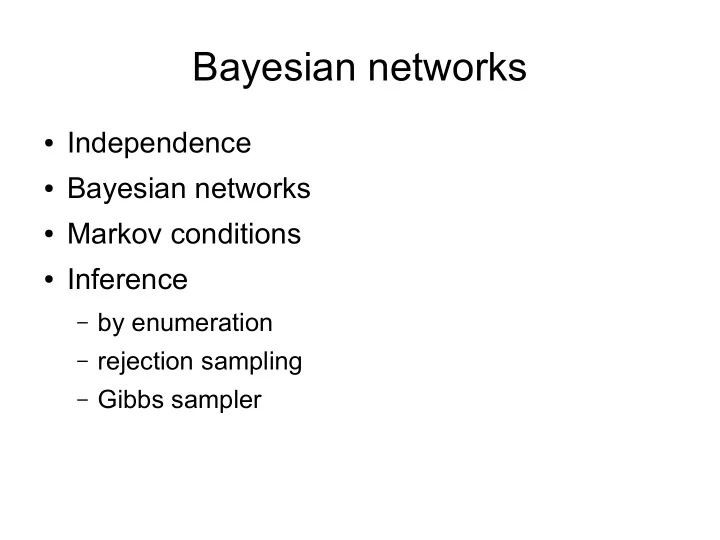
Bayesian networks Independence Bayesian networks Markov conditions - - PowerPoint PPT Presentation

• Independence
• Bayesian networks
• Markov conditions
• Inference

– by enumeration – rejection sampling – Gibbs sampler

Bayesian networks

Independence

• if P(A=a,B=a) = P(A=a)P(B=b) for all a and b,

then we call A and B (marginally) independent.

• if P(A=a,B=a | C=c) = P(A=a|C=c)P(B=b|C=c)

for all a and b, then we call A and B conditionally independent given C=c.

• if P(A=a,B=a | C=c) = P(A=a|C=c)P(B=b|C=c)

for all a, b and c, then we call A and B conditionally independent given C.

• PA ,B=PAPB

implies PA∣B=PA ,B PB =PAPB PB =PA

Independence saves space

• If A and B are independent given C
• P(A,B,C) = P(C,A,B)

= P(C)P(A|C)P(B|A,C) = P(C)P(A|C)P(B|C)

• Instead of having a full joint probability table for

P(A,B,C), we can have a table for P(C) and tables P(A|C=c) and P(B|C=c) for each c.

– Even for binary variables this saves space:

• 23 = 8 vs. 2 + 2 + 2 = 6.

– With many variables and many independences you

save a lot.

Chain Rule – Independence - BN

Chainrule : PA , B ,C , D=PAPB∣A PC∣A , B PD∣A, B ,C

A B C D A B C D A B C D

Independence: P A, B ,C , D=PAPBPC∣A , B PD∣A ,C Bayesian Network

A

But order matters

• P(A,B,C) = P(C,A,B)
• P(A)P(B|A)P(C|A,B) = P(C)P(A|C)P(B|A,C)
• And if A and B are conditionally independent

given C: 1.P(A,B,C) = P(A)P(B|A)P(C|A,B) 2.P(C,A,B) = P(C)P(A|C)P(B|C)

C B A C B

1. 2.

With the same independence assumptions, some orders yield simpler networks.

• Bayesian network structure forms a directed

acyclic graph (DAG).

• If we have a DAG G, we denote the parents of

the node (variable) Xi with PaG(xi) and a value configuration of PaG(xi) with paG(xi) :

Bayes net as a factorization

Px1,x2,..., xn∣G=∏

i=1 n

Pxi∣paGxi,

• where P(xi|paG(xi)) are called local probabilities.

– Local probabilities are stored in conditional

probability tables CPTs.

A Bayesian network

Cloudy Rain Cloudy=no Cloudy=yes 0.5 0.5 Cloudy Sprinkler=onSprinkler=off no 0.5 0.5 yes 0.9 0.1 Sprinkler Cloudy Rain=yes Rain=no no 0.2 0.8 yes 0.8 0.2 Sprinkler Rain WetGrass=yesWetGrass=no

• n

no 0.90 0.10

• n

yes 0.99 0.01

• ff

no 0.01 0.99

• ff

yes 0.90 0.10 Wet Grass

P(Cloudy) P(Sprinkler | Cloudy) P(Rain | Cloudy) P(WetGrass | Sprinkler, Rain)

Causal order recommended

• Causes first, then effects.
• Since causes render direct consequences

independent yielding smaller CPTs

• Causal CPTs are easier to assess by human

experts

• Smaller CPT:s are easier to estimate reliably

from a finite set of observations (data)

• Causal networks can be used to make causal

inferences too.

Markov conditions

• Local (parental) Markov condition

– X is independent of its ancestors given its parents.

• Global Markov Condition

– X is independent of any set of other variables given

its parents, children and parents of its children (Markov blanket)

• D-separation

– X and Y are dependent given Z, if there is an

unblocked path without colliders between X and Y.

– or if each collider or some descendant of each

collider is in Z.

Inference in Bayesian networks

• Given a Bayesian network B (i.e., DAG and

CPTs) , calculate P(X|e) where X is a set of query variables and e is an instantiaton of

• bserved variables E (X and E separate).
• There is always the way through marginals:

– normalize P(x,e) = Σy∈dom(Y)P(x,y,e), where dom(Y),

is a set of all possible instantiations of the unobserved non-query variables Y.

• There are much smarter algorithms too, but in

general the problem is NP hard.

Approximate inference in Bayesian networks

• How to estimate how probably it rains next day,

if the previous night temperature is above the month average.

– count rainy and non rainy days after warm nights

(and count relative frequencies).

• Rejection sampling for P(X|e) :

1.Generate random vectors (xr,er,yr). 2.Discard those those that do not match e. 3.Count frequencies of different xr and normalize.

How to generate random vectors from a Bayesian network

• Sample parents first

– P(C)

• (0.5, 0,5) → yes

– P(S|C=yes)

• (0.9, 0.1) → on

– P(R | C=yes)

• (0.8, 0.2) → no

– P(W | S=on, R=no)

• (0.9, 0.1) → yes
• P(C,S,R,W) =

P(yes,on,no,yes) = 0.5 x 0.9 x 0.2 x 0.9 = 0.081

Cloudy=no Cloudy=yes 0.5 0.5 Cloudy Sprinkler=onSprinkler=off no 0.5 0.5 yes 0.9 0.1 Cloudy Rain=yesRain=no no 0.2 0.8 yes 0.8 0.2 Sprinkler Rain WetGrass=yesWetGrass=no

• n

no 0.90 0.10

• n

yes 0.99 0.01

• ff

no 0.01 0.99

• ff

yes 0.90 0.10

Rejection sampling, bad news

• Good news first:

– super easy to implement

• Bad news:

– if evidence e is improbable, generated random

vectors seldom conform with e, thus it takes a long time before we get a good estimate P(X|e).

– With long E, all e are improbable.

• So called likelihood weighting can alleviate the

problem a little bit, but not enough.

Gibbs sampling

• Given a Bayesian network for n variables

X∪E∪Y, calculate P(X|e) as follows:

– N = (associative) array of zeros – Generate random vector x,y. – While True:

• for V in X,Y:

– generate v from P(V | MarkovBlanket(V)) – replace v in x,y. – N[x] +=1 – print normalize(N[x])

P(X|mb(X))?

PX∣mbX =PX∣mbx,Rest =PX ,mbX,Rest PmbX,Rest ∝PAll =∏

Xi∈X

PXi∣PaXi =PX∣PaX ∏

C∈chX

PC∣PaC

∏

R∈Rest∪PaV

PR∣PaR ∝PX∣PaX ∏

C∈chX

PC∣PaC

• All decent Markov Chains q have a unique

stationary distribution P* that can be estimated by simulation.

• Detailed balance of transition function q and

state distribution P* implies stationarity of P*.

• Proposed q, P(V|mb(V)), and P(X|e) form a

detailed balance, thus P(X|e) is a stationary distribution, so it can be estimated by simulation.

Why does it work

Markov chains stationary distribution

• Defined by transition probabilities between

states q(x→x'), where x and x' belong to a set

• f states X.
• Distribution P* over X is called stationary

distribution for the Markov Chain q, if P*(x')=∑xP*(x)q(x→x').

• P*(X) can be found out by simulating Markov

Chain q starting from the random state xr.

Markov Chain detailed balance

• Distribution P over X and a state transition

distribution q are said to form a detailed balance, if for any states x and x', P(x)q(x→x') = P(x')q(x'→x), i.e. it is equally probable to witness transition from x to x' as it is to witness transition from x' to x.

• If P and q form a detailed balance,

∑xP(x)q(x→x') = ∑xP(x')q(x'→x) = P(x')∑xq(x'→x) =P(x'), thus P is stationary.

Gibbs sampler as Markov Chain

• Consider Z=(X,Y) to be states of a Markov

chain, and q((v,z-V))→(v',z-V))=P(v'|z-V, e), where Z-V = Z-{V}. Now P*(Z)=P(Z|e) and q form a detailed balance, thus P* is a stationary distribution of q and it can be found with the sampling algorithm.

– P*(z)q(z→z') = P(z|e)P(v'|z-V, e)

= P(v,z-V|e)P(v'|z-V, e) = P(v|z-V,e)P(z-V|e)P(v'|z-V, e) = P(v|z-V,e)P(v', z-V|e) = q(z'→z)P*(z'), thus balance.