(x,y), W(y)=(y1/2) 2 1/4, =20, =0.01 1 0.9 0.8 0.7 0.6 0.5 - PowerPoint PPT Presentation

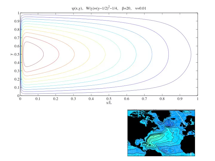
ψ (x,y), W(y)=(y−1/2) 2 −1/4, β =20, ν =0.01 1 0.9 0.8 0.7 0.6 0.5 y 0.4 0.3 0.2 0.1 0 0 0.1 0.2 0.3 0.4 0.5 0.6 0.7 0.8 0.9 1 x/L -120 - 60 0 + 60

Wind Forcing Kallberg et al. 1995 (ERA-40 reanalysis)

Ocean Currents Time-averaged (16-year) ocean circulation Wunsch, 2011 +120 ° -180 ° -120 ° - 60 ° 0 ° + 60 ° +75 ° +60 ° +45 ° 15 ° 0 ° 15 ° -45 ° -60 ° -75 ° -80 -60 -40 -20 0 20 40 60 80 100 150 200 Transport streamfunction (10 6 m 3 /s = 1 Sverdrup)

Numerical Simulations: Instantaneous Time-averaged Eddies Haidvogel, McWilliams, Gent, J. Phys. Oceanography 1992

Sea-surface temperature Instantaneous Haidvogel, McWilliams, Gent, J. Phys. Oceanography 1992 Gulf-stream ‘rings’

tracer informa- of Furthermore, for ‐ rs tem- Gouretski The surface sources of global ocean waters. Oceanic volume that has originated in each 2° by 2° surface location (11,113 origination sites), scaled by the surface area of each box to make an equivalent thickness, d. The color-scale follows a base ten logarithm of the field.

Antarctic Intermediate Water (AAIW) North Atlantic Deep Water (NADW) Antarctic Bottom Water (AABW)

Averaging, across an ocean in longitude ‣ Meridional Overturning Circulation (MOC) (sometimes called the Thermohaline Circulation, THC) Atlantic MOC (1 Sv = 10 6 m 3 /s) − 30 − 27 21 30 − 24 − 3 30 2 0 9 6 − 18 − 21 7 − 15 − 12 4 6 9 3 − 6 − − 3 15 0 21 21 2 9 3 1 12 6 9 1 18 24 2 1 21 2 0 1 3 8 18 24 15 3 15 2 − 15 21 12 15 9 3 − 1000 12 − 3 21 − 6 6 − 12 − 9 15 18 9 12 15 12 6 9 − 3 − 3 12 3 0 − 6 6 − 2000 Depth, (m) 3 − 6 6 9 0 3 9 0 − 3 3 6 0 − 12 6 3 − 6 − − 3 − − 3 9 − 6 0 − 18 − 30 − 21 − 24 − 27 − 15 0 3 0 8 0 1 7 4 5 − 3000 2 1 2 2 3 1 0 − 12 − − − − − − − 6 − 9 − 9 − 6 − 3 − 3 6 − 3 − 6 3 − − 12 9 − 9 − − 0 9 0 0 − 21 − 30 − 18 − 27 − 15 − 24 − 12 − 3 − 9 − 6 3 − − 4000 0 6 − − 6 − 3 − 3 0 − 3 0 0 0 − 24 − 27 − 21 − 15 − 18 − 30 − 5000 − 60 − 40 − 20 0 20 40 60 Latitude Nikurashin and Vallis, 2011

Mignotti + Woods, 2015

Mixed layer MI Thermocline THERMO PYCNOCLI Abyss ABYSS

S N Eq. 0 26.6 26.8 26.7 25 26 26.6 27.2 26.7 26.9 26 26.5 27 26.8 26.9 26.5 26.6 27.3 27 26.7 26.8 500 27.1 26.9 27.1 27.2 27.7 27.72 27 27.2 27.3 27.4 27.1 27.3 27.4 27.4 27.5 27.5 27.54 27.2 27.56 27.52 27.3 27.4 1000 27.58 27.64 27.62 27.74 27.5 27.52 27.6 27.54 27.52 27.5 27.58 27.54 27.56 27.52 27.54 27.7 27.56 27.58 27.62 27.66 27.6 27.56 27.6 27.64 27.58 27.68 27.6 27.68 27.72 27.62 27.66 27.76 27.62 27.66 27.64 27.7 27.78 27.74 27.66 27.72 27.68 27.82 1500 27.64 27.7 27.74 27.8 27.68 27.72 27.74 27.76 27.76 27.82 27.78 27.76 27.84 27.7 27.8 27.72 27.78 2000 27.8 27.82 27.76 27.78 27.74 27.86 27.78 27.84 27.84 27.8 27.8 27.82 27.82 2500 27.84 27.86 27.86 27.86 27.88 3000 27.82 27.88 27.84 3500 27.88 27.84 4000 4500 27.86 27.88 27.86 5000 27.86 5500 27.68 27.66 27.62 27.76 27.64 27.78 27.74 27.72 27.58 27.54 27.82 27.84 27.56 27.52 27.6 27.7 27.8 26.5 26.9 26.6 26.8 26.7 27.1 27.2 27.3 27.5 27.4 27 26 20 22 21 23 24 25 27.76 27.74 27.78 27.84 27.82 27.72 27.64 27.58 27.68 27.62 27.54 27.56 27.66 27.52 27.8 27.6 27.7 26.8 27.1 26.6 27.2 27.3 27.5 26.5 26.9 26.7 27.4 27 26 27.88 27.68 27.64 27.52 27.54 27.72 27.56 27.84 27.82 27.62 27.74 27.58 27.76 27.66 27.78 27.1 26.9 26.5 27.2 26.8 27.6 26.7 27.7 27.3 27.4 26.6 27.8 27.5 24 20 21 25 27 23 26 22 27.86 27.88 6000 km 0 1000 2000 3000 4000 5000 6000 7000 8000 9000 10000 11000 12000 13000 Lat -50 -40 -30 -20 -10 0 10 20 30 40 50 60

‘Missing’ Mixing Problem: Observations of ocean mixing typically find Inferred diffusivity, North-South Atlantic section Munk value Kunze et al. JPO, 2006

κ T ' 1 . 1 ⇥ 10 − 5 m 2 s − 1

Mixing Efficiency Inoue + Smyth 2009