SLIDE 1 Workshop 10: Non-linear Regression
Murray Logan 26-011-2013 Linear models
LM y ∼ N(µ, σ2) µ = β0 + β1x1 + β2x2 Polynomial y ∼ N(µ, σ2) µ = β0 + β1x + β2x2 + β2x3
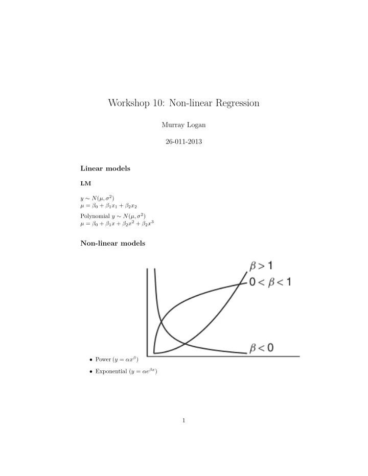
Non-linear models
- Power (y = αxβ)
- Exponential (y = αeβx)
1
SLIDE 2 Non-linear models
- Asymptotic exponential y = α+(β−α)e−eγx
- Michaelis-Menton (y =
αx β+x)
2
SLIDE 3 Non-linear models
nls(y ~ a * exp(b * x), start = list(a = 1, b = 1))
Linear models
LM y ∼ N(µ, σ2) µ = β0 + β1x1 + β2x2 GLM y ∼ Pois(µ, σ2) g(µ) = β0 + β1x1 + β2x2
Linear models
- only permit parametric non-linearity
– polynomials – nls
Examples
peake <- read.table("../data/peake.csv", header = T, sep = ",", strip.white = T) head(peake) AREA SPECIES INDIV 1 516.0 3 18 2 469.1 7 60 3 462.2 6 57 4 938.6 8 100 5 1357.2 10 48 6 1773.7 9 118 ## @knitr Q4-a, fig.height=5.0, fig.width=5.0 library(car) scatterplot(SPECIES ~ AREA, data = peake) 3
SLIDE 4
Figure 1: plot of chunk unnamed-chunk-1 4
SLIDE 5
## @knitr Q4-2a peake.lm <- lm(SPECIES ~ AREA + I(AREA^2), data = peake) ## @knitr Q4-2b peake.nls <- nls(SPECIES ~ alpha * AREA^beta, data = peake, start = list(alpha = 0.1, beta = 1)) ## @knitr Q4-2c peake.nls1 <- nls(SPECIES ~ SSasymp(AREA, a, b, c), data = peake) ## @knitr Q4-3a peake.lmLin <- lm(SPECIES ~ AREA, data = peake) # calculate AIC for the linear model AIC(peake.lmLin) [1] 141.1 # calculate mean-square residual of the linear # model deviance(peake.lmLin)/df.residual(peake.lmLin) [1] 14.13 AIC(peake.lm) [1] 129.5 # calculate mean-square residual of the power model deviance(peake.lm)/df.residual(peake.lm) [1] 8.602 # assess the goodness of fit between linear and # polynomial models anova(peake.lmLin, peake.lm) 5
SLIDE 6
Analysis of Variance Table Model 1: SPECIES ~ AREA Model 2: SPECIES ~ AREA + I(AREAˆ2) Res.Df RSS Df Sum of Sq F Pr(>F) 1 23 325 2 22 189 1 136 15.8 0.00064 * — Signif. codes: 0 ‘’ 0.001 ’’ 0.01 ’’ 0.05 ’.’ 0.1 ’ ’ 1 # calculate AIC for the exponential asymptotic # model AIC(peake.nls) [1] 125.1 # calculate mean-square residual of the exponential # asymptotic model deviance(peake.nls)/df.residual(peake.nls) [1] 7.469 # calculate AIC for the exponential asymptotic # model AIC(peake.nls1) [1] 125.8 # calculate mean-square residual of the exponential # asymptotic model deviance(peake.nls1)/df.residual(peake.nls1) [1] 7.393 # assess the goodness of fit between polynomial and # power models anova(peake.nls, peake.nls1) Analysis of Variance Table Model 1: SPECIES ~ alpha * AREAˆbeta Model 2: SPECIES ~ SSasymp(AREA, a, b, c) Res.Df Res.Sum Sq Df Sum Sq F value Pr(>F) 1 23 172 2 22 163 1 9.14 1.24 0.28 6
SLIDE 7
- par <- par(mfrow = c(2, 2), mar = c(5, 5, 0, 0))
# first plot linear trend
- par1 <- par(mar = c(5, 5, 0, 0))
plot(SPECIES ~ AREA, data = peake, ann = F, axes = F, type = "n") points(SPECIES ~ AREA, data = peake, col = "grey", pch = 16) xs <- with(peake, seq(min(AREA), max(AREA), l = 1000)) ys <- predict(peake.lmLin, data.frame(AREA = xs), interval = "confidence") points(ys[, "fit"] ~ xs, col = "black", type = "l") points(ys[, "lwr"] ~ xs, col = "black", type = "l", lty = 2) points(ys[, "upr"] ~ xs, col = "black", type = "l", lty = 2) axis(1, cex.axis = 0.75) mtext(expression(paste("Clump area", (dm^2))), 1, line = 3, cex = 1.2) axis(2, las = 1, cex.axis = 0.75) mtext(expression(paste("Number of species (", phantom() %+-% 95, "%CI)")), 2, line = 3, cex = 1.2) box(bty = "l") par(opar1) # second plot polynomial trend
- par1 <- par(mar = c(5, 5, 0, 0))
plot(SPECIES ~ AREA, data = peake, ann = F, axes = F, type = "n") points(SPECIES ~ AREA, data = peake, col = "grey", pch = 16) xs <- with(peake, seq(min(AREA), max(AREA), l = 1000)) ys <- predict(peake.lm, data.frame(AREA = xs), interval = "confidence") points(ys[, "fit"] ~ xs, col = "black", type = "l") points(ys[, "lwr"] ~ xs, col = "black", type = "l", lty = 2) points(ys[, "upr"] ~ xs, col = "black", type = "l", lty = 2) axis(1, cex.axis = 0.75) mtext(expression(paste("Clump area", (dm^2))), 1, line = 3, cex = 1.2) axis(2, las = 1, cex.axis = 0.75) mtext(expression(paste("Number of species (", phantom() %+-% 95, "%CI)")), 2, line = 3, cex = 1.2) box(bty = "l") par(opar1)
- par1 <- par(mar = c(5, 5, 0, 0))
7
SLIDE 8 plot(SPECIES ~ AREA, data = peake, ann = F, axes = F, type = "n") points(SPECIES ~ AREA, data = peake, col = "grey", pch = 16) xs <- with(peake, seq(min(AREA), max(AREA), l = 1000)) ys <- predict(peake.nls1, data.frame(AREA = xs)) se.fit <- sqrt(apply(attr(ys, "gradient"), 1, function(x) sum(vcov(peake.nls1) *
points(ys ~ xs, col = "black", type = "l") points(ys + 2 * se.fit ~ xs, col = "black", type = "l", lty = 2) points(ys - 2 * se.fit ~ xs, col = "black", type = "l", lty = 2) axis(1, cex.axis = 0.75) mtext(expression(paste("Clump area", (dm^2))), 1, line = 3, cex = 1.2) axis(2, las = 1, cex.axis = 0.75) mtext(expression(paste("Number of species", (phantom() %+-% 2 ~ SE), )), 2, line = 3, cex = 1.2) box(bty = "l") par(opar1) # we need to refit the model in order to get # gradient calculations from which se can be # calculated this requires that the gradient be # specified using the deriv3() function. grad <- deriv3(~alpha * AREA^beta, c("alpha", "beta"), function(alpha, beta, AREA) NULL) peake.nls <- nls(SPECIES ~ grad(alpha, beta, AREA), data = peake, start = list(alpha = 0.1, beta = 1)) ys <- predict(peake.nls, data.frame(AREA = xs)) se.fit <- sqrt(apply(attr(ys, "gradient"), 1, function(x) sum(vcov(peake.nls) *
- uter(x, x))))
- par1 <- par(mar = c(5, 5, 0, 0))
plot(SPECIES ~ AREA, data = peake, ann = F, axes = F, type = "n") points(SPECIES ~ AREA, data = peake, col = "grey", pch = 16) points(ys ~ xs, col = "black", type = "l") # 2*SE equates approximately to 95% confidence # intervals technically it is qt(0.975,df)*SE # therefore this could also be labeled as 90%CI points(ys + 2 * se.fit ~ xs, col = "black", type = "l", lty = 2) points(ys - 2 * se.fit ~ xs, col = "black", type = "l", 8
SLIDE 9 lty = 2) axis(1, cex.axis = 0.75) mtext(expression(paste("Clump area", (dm^2))), 1, line = 3, cex = 1.2) axis(2, las = 1, cex.axis = 0.75) mtext(expression(paste("Number of species", (phantom() %+-% 2 ~ SE), )), 2, line = 3, cex = 1.2) box(bty = "l") Figure 2: plot of chunk unnamed-chunk-1
Smoothers / splines
- allow non-parametric non-linearity
9
SLIDE 10
- piecewise polynomial functions
Piecewise regression
Figure 3:
Piecewise regression Smoothers / splines
- allow non-parametric non-linearity
- piecewise polynomial functions
- joined by knots
10
SLIDE 11
Figure 4: 11
SLIDE 12 Piecewise regression
Figure 5:
Piecewise regression Piecewise regression
yi = β0 + β1(xi) + β2(xi − cp) yi = β0 + β1I(xi < xcp)(xi) + β2I(xi > xcp)(xi − xcp)
- single knot
- determined by hypothesis
12
SLIDE 13
Figure 6: 13
SLIDE 14 Cubic spline
Figure 7:
Smoother
- a function that relates Y to one or more X’s
- types of smoothers
– polynomials (parametric) – lowess, loess – splines ∗ cubic ∗ thin-plate 14
SLIDE 15 Smoother
– no parameters – must be plotted to explore relationship
Smoother - lowess
Figure 8: 15
SLIDE 16 Degree of smoothing
– under and over smoothing – describe trend without focusing on outliers
- model fit (residual sum of squares)
- penalized for degree of smoothing (wiggliness)
Degree of smoothing
Generalized Cross-validation
- create as many subsets as their are observations
- fit all models with all λ
- select best λ
Generalized Additive Models
LM y ∼ N(µ, σ2) µ = β0 + β1x1 + β2x2 GLM y ∼ Pois(µ, σ2) g(µ) = β0 + β1x1 + β2x2
Generalized Additive Models
GLM y ∼ Pois(µ, σ2) g(µ) = β0 + β1x1 + β2x2 GAM y ∼ Pois(µ, σ2) g(µ) = β0 + f(x1) + f(x2) 16
SLIDE 17 Generalized Additive Models
- allow multiple predictors (each with own smoothing function)
- assume pure additivity (no interactions)
GAM
library(mgcv) dat.gam <- gam(y ~ s(x1) + s(x2) + s(x3), data = dat) summary(dat.gam)
GAM
Family: gaussian Link function: identity Formula: y ~ s(x1) + s(x2) + s(x3) Parametric coefficients: Estimate Std. Error t value Pr(>|t|) (Intercept) 7.948 0.109 72.7 <2e-16 (Intercept) ***
0 ’***’ 0.001 ’**’ 0.01 ’*’ 0.05 ’.’ 0.1 ’ ’ 1 Approximate significance of smooth terms: edf Ref.df F p-value s(x1) 3.00 3.71 70.04 <2e-16 *** s(x2) 8.09 8.77 75.02 <2e-16 *** s(x3) 5.05 6.15 3.25 0.0037 **
0 ’***’ 0.001 ’**’ 0.01 ’*’ 0.05 ’.’ 0.1 ’ ’ 1 R-sq.(adj) = 0.692 Deviance explained = 70.5% GCV score = 5.0027 Scale est. = 4.7884 n = 400
GAM
plot(dat.gam, pages = 1) 17
SLIDE 18
Figure 9:
GAM
plot(dat.gam, select = 2, shade = TRUE)
GAM
Interactions library(mgcv) dat.gam <- gam(y ~ s(x2, x3), data = dat) summary(dat.gam) 18
SLIDE 19
Figure 10: 19
SLIDE 20 GAM
Family: gaussian Link function: identity Formula: y ~ s(x2, x3) Parametric coefficients: Estimate Std. Error t value Pr(>|t|) (Intercept) 7.948 0.144 55.3 <2e-16 (Intercept) ***
0 ’***’ 0.001 ’**’ 0.01 ’*’ 0.05 ’.’ 0.1 ’ ’ 1 Approximate significance of smooth terms: edf Ref.df F p-value s(x2,x3) 24.4 27.8 12.8 <2e-16 ***
0 ’***’ 0.001 ’**’ 0.01 ’*’ 0.05 ’.’ 0.1 ’ ’ 1 R-sq.(adj) = 0.47 Deviance explained = 50.2% GCV score = 8.8159 Scale est. = 8.2553 n = 400
GAM
plot(dat.gam, pages = 1, scheme = 2)
GAM
vis.gam(dat.gam, theta = 35)
GAM
vis.gam(dat.gam, theta = 35, se = 2) 20
SLIDE 21
Figure 11: 21
SLIDE 22
Figure 12: 22
SLIDE 23
Figure 13: 23
SLIDE 24
Worked Examples
peake <- read.table("../data/peake.csv", header = T, sep = ",", strip.white = T) head(peake) AREA SPECIES INDIV 1 516.0 3 18 2 469.1 7 60 3 462.2 6 57 4 938.6 8 100 5 1357.2 10 48 6 1773.7 9 118 24