SLIDE 1 Working with tidy data in R: tidyverse
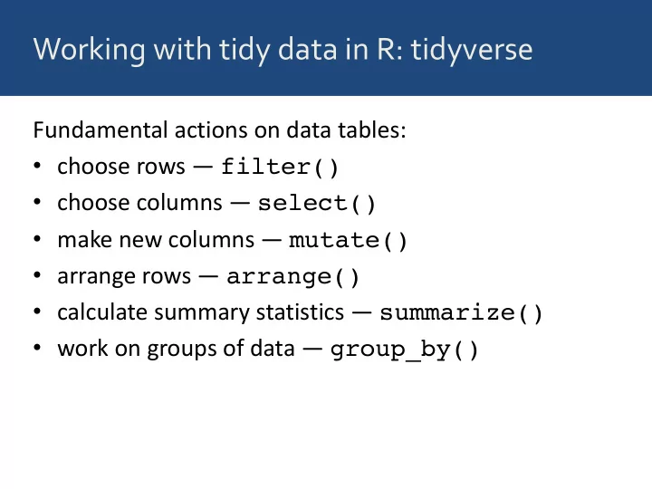
Fundamental actions on data tables:
- choose rows — filter()
- choose columns — select()
- make new columns — mutate()
- arrange rows — arrange()
- calculate summary statistics — summarize()
- work on groups of data — group_by()
SLIDE 2 We can combine these verbs using the pipe
Standard R: > mean(iris$Sepal.Length) [1] 5.843333 With pipe: > iris$Sepal.Length %>% mean() [1] 5.843333
SLIDE 3 We can combine these verbs using the pipe
Standard R:
> head(iris) Sepal.Length Sepal.Width Petal.Length Petal.Width Species 1 5.1 3.5 1.4 0.2 setosa 2 4.9 3.0 1.4 0.2 setosa 3 4.7 3.2 1.3 0.2 setosa 4 4.6 3.1 1.5 0.2 setosa 5 5.0 3.6 1.4 0.2 setosa 6 5.4 3.9 1.7 0.4 setosa
SLIDE 4 We can combine these verbs using the pipe
With pipe:
> iris %>% head() Sepal.Length Sepal.Width Petal.Length Petal.Width Species 1 5.1 3.5 1.4 0.2 setosa 2 4.9 3.0 1.4 0.2 setosa 3 4.7 3.2 1.3 0.2 setosa 4 4.6 3.1 1.5 0.2 setosa 5 5.0 3.6 1.4 0.2 setosa 6 5.4 3.9 1.7 0.4 setosa
SLIDE 5
Combining pipe and assignment
These two lines do the same thing:
> mean_length <- mean(iris$Sepal.Length) > mean_length <- iris$Sepal.Length %>% mean() > mean_length [1] 5.843333
SLIDE 6 Pipe example 1: count how many herbivores
- f different orders there are in msleep
SLIDE 7 Pipe example 1: count how many herbivores
- f different orders there are in msleep
msleep %>% filter(vore == "herbi")
SLIDE 8 Pipe example 1: count how many herbivores
- f different orders there are in msleep
msleep %>% filter(vore == "herbi") %>% group_by(order)
SLIDE 9 Pipe example 1: count how many herbivores
- f different orders there are in msleep
msleep %>% filter(vore == "herbi") %>% group_by(order) %>% summarize(count = n())
SLIDE 10 Pipe example 1: count how many herbivores
- f different orders there are in msleep
msleep %>% filter(vore == "herbi") %>% group_by(order) %>% summarize(count = n()) %>% arrange(desc(count))
SLIDE 11 Pipe example 1: count how many herbivores
- f different orders there are in msleep
msleep %>% filter(vore == "herbi") %>% group_by(order) %>% summarize(count = n()) %>% arrange(desc(count))
1 Rodentia 16 2 Artiodactyla 5 3 Perissodactyla 3 4 Hyracoidea 2 5 Proboscidea 2 6 Diprotodontia 1 7 Lagomorpha 1 8 Pilosa 1 9 Primates 1
SLIDE 12
Pipe example 2: What is total day time for each animal in msleep?
SLIDE 13
Pipe example 2: What is total day time for each animal in msleep?
msleep %>% mutate(total_day_time = awake + sleep_total)
SLIDE 14
Pipe example 2: What is total day time for each animal in msleep?
msleep %>% mutate(total_day_time = awake + sleep_total) %>% select(name, total_day_time)
SLIDE 15
Pipe example 2: What is total day time for each animal in msleep?
msleep %>% mutate(total_day_time = awake + sleep_total) %>% select(name, total_day_time) name total_day_time 1 Cheetah 24.00 2 Owl monkey 24.00 3 Mountain beaver 24.00 4 Greater short-tailed shrew 24.00 5 Cow 24.00 6 Three-toed sloth 24.00 7 Northern fur seal 24.00 8 Vesper mouse 24.00 9 Dog 24.00 10 Roe deer 24.00
SLIDE 16
Pipe example 3: What is the median awake time of different orders in msleep?
SLIDE 17
Pipe example 3: What is the median awake time of different orders in msleep?
msleep %>% group_by(order)
SLIDE 18
Pipe example 3: What is the median awake time of different orders in msleep?
msleep %>% group_by(order) %>% summarize(med_awake = median(awake))
SLIDE 19
Pipe example 3: What is the median awake time of different orders in msleep?
msleep %>% group_by(order) %>% summarize(med_awake = median(awake)) %>% arrange(med_awake)
SLIDE 20 Pipe example 3: What is the median awake time of different orders in msleep?
msleep %>% group_by(order) %>% summarize(med_awake = median(awake)) %>% arrange(med_awake)
1 Chiroptera 4.20 2 Didelphimorphia 5.30 3 Cingulata 6.25 4 Afrosoricida 8.40 5 Pilosa 9.60 6 Rodentia 11.10 7 Diprotodontia 11.60 8 Soricomorpha 13.70 9 Carnivora 13.75 10 Erinaceomorpha 13.80