Words in Context Sense Examples (keyword in context) . . . used to - - PowerPoint PPT Presentation

6.864 (Fall 2007)

Word-Sense Disambiguation, and Semi-Supervised Learning

1

Overview

• A supervised method for word-sense disambiguation: decision

lists

• A semi-supervised method for word-sense disambiguation
• A semi-supervised method for named-entity classification

2

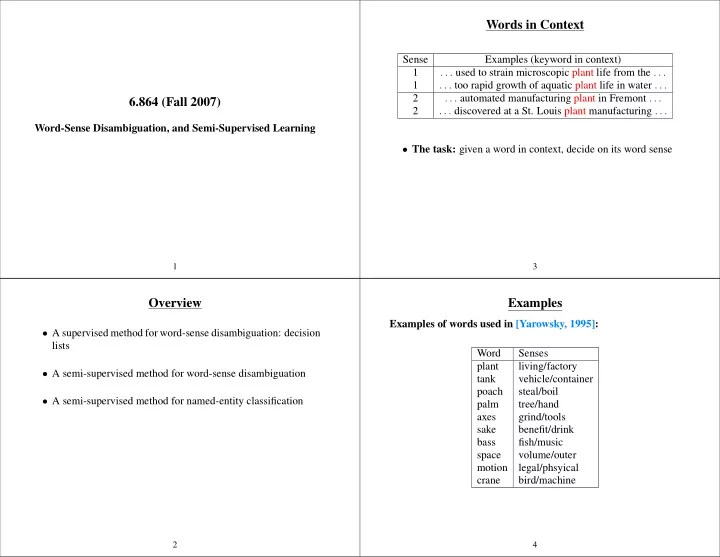
Words in Context

Sense Examples (keyword in context) 1 . . . used to strain microscopic plant life from the . . . 1 . . . too rapid growth of aquatic plant life in water . . . 2 . . . automated manufacturing plant in Fremont . . . 2 . . . discovered at a St. Louis plant manufacturing . . .

• The task: given a word in context, decide on its word sense

3

Examples

Examples of words used in [Yarowsky, 1995]: Word Senses plant living/factory tank vehicle/container poach steal/boil palm tree/hand axes grind/tools sake benefit/drink bass fish/music space volume/outer motion legal/phsyical crane bird/machine

4

Features Used in the Model

• Word found in +/ − k word window
• Word immediately to the right (+1 W)
• Word immediately to the left (-1 W)
• Pair of words at offsets -2 and -1
• Pair of words at offsets -1 and +1
• Pair of words at offsets +1 and +2

5

Features Used in the Model

• Also maps words to parts of speech, and general classes (e.g.,

WEEKDAY, MONTH etc.)

• Local features including word classes are added:

– Pair of tags at offsets -2 and -1 – Tag at position -2, word at position -1 – etc.

6

An Example

The ocean reflects the color of the sky, but even on cloudless days the color of the ocean is not a consistent blue. Phytoplankton, microscopic plant life that floats freely in the lighted surface waters, may alter the color of the water. When a great number of organisms are concentrated in an area, the plankton changes the color of the

• cean surface. This is called a ’bloom.’

⇓

w−1 = Phytoplankton t−1 = JJ w+1 = life t+1 = NN w−2, w−1 = (Phytoplankton,microscopic) t−2, t−1 = (NN,JJ) w−1, w+1 = (microscopic,life) . . . w+1, w+2 = (life,that) word-within-k = ocean word-within-k = reflects word-within-k = color . . . word-within-k = bloom 7

A Machine-Learning Method: Decision Lists

• For each feature, we can get an estimate of conditional

probability of sense 1 and sense 2

• For example, take the feature w+1 =life
• We might have

Count(sense 1 of plant, w+1 =life) = 100 Count(sense 2 of plant, w+1 =life) = 1

• Maximum-likelihood estimate

P(sense 1 of plant | w+1 =life) = 100 101

8

Smoothed Estimates

• Usual problem: some counts are sparse
• We might have

Count(sense 1 of plant, w−1 =Phytoplankton) = 2 Count(sense 2 of plant, w−1 =Phytoplankton) =

• α smoothing (empirically, α ≈ 0.1 works well):

P(sense 1 of plant | w−1 =Phytoplankton) = 2 + α 2 + 2α P(sense 1 of plant | w+1 =life) = 100 + α 101 + 2α with α = 0.1, gives values of 0.95 and 0.99 (unsmoothed gives values of 1 and 0.99) 9

Creating a Decision List

• For each feature, find

sense(feature) = argmaxsenseP(sense | feature) e.g., sense(w+1 =life) = sense1

• Create a rule feature → sense(feature) with weight

P(sense(feature) | feature). e.g.,

Rule Weight w+1 =life → sense 1 0.99 w−1 =Phytoplankton → sense 1 0.95 . . . 10

Creating a Decision List

• Create a list of rules sorted by strength

Rule Weight w+1 =life → sense 1 0.99 w−1 =manufacturing → sense 2 0.985 word-within-k=life → sense 1 0.98 word-within-k=manufacturing → sense 2 0.979 word-within-k=animal → sense 1 0.975 word-within-k=equipment → sense 2 0.97 word-within-k=employee → sense 2 0.968 w−1 =assembly → sense 2 0.965 . . .

• To apply the decision list: take the fi rst (strongest) rule in the list which

applies to an example 11

The ocean refl ects the color of the sky, but even on cloudless days the color

• f the ocean is not a consistent blue. Phytoplankton, microscopic plant life

that fl

• ats freely in the lighted surface waters, may alter the color of the
• water. When a great number of organisms are concentrated in an area, the

plankton changes the color of the ocean surface. This is called a ’bloom.’

Feature Sense Strength w−1 = Phytoplankton 1 0.95 w+1 = life 1 0.99 w−2, w−1 = (Phytoplankton,microscopic) N/A w−1, w+1 = (microscopic,life) N/A w+1, w+2 = (life,that) 1 0.96 word-within-k = ocean 1 0.93 word-within-k = reflects N/A word-within-k = color 2 0.65 t−1 = JJ 2 0.56 t−2, t−1 = (NN,JJ) 2 0.7 t+1 = NN 1 0.64 . . .

• N/A ⇒ feature has not been seen in training data
• w+1 = life → Sense 1 is chosen

12

Experiments

• [Yarowsky, 1994] applies the method to accent restoration in

French, Spanish

De-accented form Accented form Percentage cesse cesse 53% cess´ e 47% coute coˆ ute 53% coˆ ut´ e 47% cote cˆ

• t´

e 69% cˆ

• te

28% cote 3% cot´ e < 1%

• Task is to recover accents on words

– Very easy to collect training/test data – Very similar task to word-sense disambiguation – Useful for restoring accents in de-accented text,

• r in automatic generation of accents while typing

13

Overview

• A supervised method for word-sense disambiguation: decision

lists

• A semi-supervised method for word-sense disambiguation
• A semi-supervised method for named-entity classification

14

A Partially Supervised Method

• Collecting labeled data can be expensive
• We’ll now describe an approach that uses a small amount of

labeled data, and a large amount of unlabeled data

15

A Key Property: Redundancy

The ocean reflects the color of the sky, but even on cloudless days the color of the ocean is not a consistent blue. Phytoplankton, microscopic plant life that floats freely in the lighted surface waters, may alter the color of the water. When a great number of organisms are concentrated in an area, the plankton changes the color of the

• cean surface. This is called a ’bloom.’

⇓

w−1 = Phytoplankton word-within-k = ocean w+1 = life word-within-k = reflects w−2, w−1 = (Phytoplankton,microscopic) word-within-k = bloom w−1, w+1 = (microscopic,life) word-within-k = color w+1, w+2 = (life,that) . . .

There are often many features which indicate the sense of the word

16

Another Useful Property: “One Sense per Discourse”

• Yarowsky observes that if the same word appears more than
• nce in a document, then it is very likely to have the same

sense every time

17

Step 1 of the Method: Collecting Seed Examples

• Goal: start with a small subset of the training data being

labeled

• Various methods for achieving this:

– Label a number of training examples by hand – Pick a single feature for each class by hand e.g., word-within-k=bird and word-within-k=machinery for crane – Look through frequently occurring features, and label a few of them – Using words in dictionary defi nitions e.g., Pick words in the two defi nitions for “plant” A vegetable organism, or part of one, ready for planting or lately planted. equipment, machinery, apparatus, for an industrial activity 18

An example: for the “plant” sense distinction, initial seeds are word-within-k=life and word-within-k=manufacturing Partitions the unlabeled data into three sets:

• 82 examples labelled with “life” sense
• 106 examples labelled with “manufacturing” sense
• 7350 unlabeled examples

19

Training New Rules

• 1. From the seed data, learn a decision list of all rules with weight

above some threshold (e.g., all rules with weight > 0.97)

• 2. Using the new rules, relabel the data

(usually we will now end up with more data being labeled)

• 3. Induce a new set of rules with weight above the threshold from

the labeled data

• 4. If some examples are still not labeled, return to step 2

20

Experiments

• Yarowsky describes several experiments:

– A baseline score for just picking the most frequent sense for each word – Score for a fully supervised method – Partially supervised method with “two words” as a seed – Partially supervised method with dictionary defn. as a seed – Partially supervised method with hand-chosen rules as a seed – Dictionary defn. method combined with one-sense-per-discourse constraint 21

• ✁

• ✄

• ☎

• ✆

• ✝

• ✞

• ✟

• ✠

• ✡

• ✁

• ✁

• ✟

• ✘

22

Some Comments

• Very impressive results using relatively little supervision
• How well would this perform on words with “weaker” sense

distinctions? (e.g., interest)

• Can we give formal guarantees for when this method

will/won’t work? (how to give a formal characterization of redundancy, and show that this implies guarantees concerning the utility of unlabeled data?)

• There are several “tweakable” parameters of the method

(e.g., the weight threshold used to filter the rules)

• Another issue: the method as described may not ever label all

examples

23

Overview

• A supervised method for word-sense disambiguation: decision

lists

• A semi-supervised method for word-sense disambiguation
• A semi-supervised method for named-entity classification

24

Supervised Learning

• We have domains X, Y
• We have labeled examples (xi, yi) for i = 1 . . . n
• Task is to learn a function F : X → Y

25

Statistical Assumptions

• We have domains X, Y
• We have labeled examples (xi, yi) for i = 1 . . . n
• Task is to learn a function F : X → Y
• Typical assumption is that there is some distribution P(x, y)

from which examples are drawn

• Aim is to find a function F with a low value for

Er(F) =

• x,y

P(x, y)[[F(x) = y]] i.e., minimize probability of error on new examples

26

Partially Supervised Learning

• We have domains X, Y
• We have labeled examples (xi, yi) for i = 1 . . . n

(n is typically small)

• We have unlabeled examples (xi) for i = (n + 1) . . . (n + m)
• Task is to learn a function F : X → Y
• New questions:

– Under what assumptions is unlabeled data “useful”? – Can we fi nd NLP problems where these assumptions hold? – Which algorithms are suggested by the theory? 27

Named Entity Classification

• Classify entities as organizations, people or locations

Steptoe & Johnson = Organization

• Mrs. Frank

= Person Honduras = Location

• Need to learn (weighted) rules such as

contains(Mrs.) ⇒ Person full-string=Honduras ⇒ Location context=company ⇒ Organization

28

An Approach Using Minimal Supervision

• Assume a small set of “seed” rules

contains(Incorporated) ⇒ Organization full-string=Microsoft ⇒ Organization full-string=I.B.M. ⇒ Organization contains(Mr.) ⇒ Person full-string=New York ⇒ Location full-string=California ⇒ Location full-string=U.S. ⇒ Location

• Assume a large amount of unlabeled data

.., says Mr. Cooper, a vice president of ...

• Methods gain leverage from redundancy:

Either Spelling or Context alone is often sufficient to determine an entity’s type

29

Cotraining (Blum and Mitchell, 1998)

• We have domains X, Y
• We have labeled examples (xi, yi) for i = 1 . . . n
• We have unlabeled examples (xi) for i = (n + 1) . . . (n + m)
• We assume each example xi splits into two views, x1i and x2i
• e.g., if xi is a feature vector in R2d, then x1i and x2i are

representations in Rd.

30

The Data

• Approx 90,000 spelling/context pairs collected
• Two types of contexts identified by a parser
• 1. Appositives

.., says Mr. Cooper, a vice president of ...

• 2. Prepositional Phrases

Robert Haft , president of the Dart Group Corporation ...

31

Features: Two Views of Each Example

.., says Mr. Cooper, a vice president of ... ⇓ Spelling Features Contextual Features Full-String = Mr. Cooper appositive = president Contains(Mr.) Contains(Cooper)

32

Two Assumptions Behind Cotraining

Assumption 1: Either view is sufficient for learning There are functions F 1 and F 2 such that F(x) = F 1(x1) = F 2(x2) = y for all (x, y) pairs

33

Examples of Problems with Two Natural Views

• Named entity classification (spelling vs. context)
• Web page classification [Blum and Mitchell, 1998]

One view = words on the page, other view is pages linking to a page

• Word sense disambiguation: a random split of the text?

34

A Key Property: Redundancy

The ocean reflects the color of the sky, but even on cloudless days the color of the ocean is not a consistent blue. Phytoplankton, microscopic plant life that floats freely in the lighted surface waters, may alter the color of the water. When a great number of organisms are concentrated in an area, the plankton changes the color of the

• cean surface. This is called a ’bloom.’

⇓

w−1 = Phytoplankton word-within-k = ocean w+1 = life word-within-k = reflects w−2, w−1 = (Phytoplankton,microscopic) word-within-k = bloom w−1, w+1 = (microscopic,life) word-within-k = color w+1, w+2 = (life,that) . . .

There are often many features which indicate the sense of the word

35

Two Assumptions Behind Cotraining

Assumption 2: Some notion of independence between the two views

e.g., The Conditional-independence-given-label assumption: If P(x1, x2, y) is the distribution over examples, then P(x1, x2, y) = P0(y)P1(x1 | y)P2(x2 | y) for some distributions P0, P1 and P2 36

Why are these Assumptions Useful?

• Two examples/scenarios:

– Rote learning, and a graph interpretation – Constraints on hypothesis spaces

37

Rote Learning, and a Graph Interpretation

• In a rote learner, functions F 1 and F 2 are look-up tables

Spelling Category Robert-Jordan PERSON Washington LOCATION Washington LOCATION Jamie-Gorelick PERSON Jerry-Jasinowski PERSON Pacifi Corp COMPANY . . . . . . Context Category partner PERSON partner-at COMPANY law-in LOCATION fi rm-in LOCATION partner PERSON partner-of COMPANY . . . . . .

• Note: this can be a very inefficient learning method

(no chance to learn generalizations such as “any name containing Mr. is a person”) 38

Rote Learning, and a Graph Interpretation

• Each node in the graph is a spelling or context

A node for Robert Jordan, Washington, law-in, partner etc.

• Each (x1i, x2i) pair is an edge in the graph

e.g., (Robert Jordan, partner)

• An edge between two nodes mean they have the same label

(relies on assumption 1: each view is sufficient for classification)

• As quantity of unlabeled data increases, graph becomes more

connected (relies on assumption 2: some independence between the two views)

39

Constraints on Hypothesis Spaces

• n + m training examples xi = (x1i, x2i)
• First n examples have labels yi
• Learn functions F 1 and F 2 such that

F 1(x1i) = F 2(x2i) = yi i = 1 . . . n F 1(x1i) = F 2(x2i) i = n + 1 . . . n + m

• The second set of constraints is new, and may significantly

restrict the set of possible functions F 1 and F 2. This may significantly reduce the number of labeled examples, n, that are required for accurate learning.

40

A Linear Model

• How to build a classifier from spelling features alone?

A linear model:

– GEN(x1) is possible labels {person, location, organization} – f(x1, y) is a set of features on spelling/label pairs, e.g., f 100(x1, y) = 1 if x1 contains Mr., and y = person

• therwise

f 101(x1, y) = 1 if x1 is IBM, and y = person

• therwise

– w is parameter vector, as usual choose F 1(x1, w) = arg max

y∈GEN(x1) f(x1, y) · w

– ⇒ each parameter in w gives a weight for a feature/label pair. e.g., w100 = 2.5, w101 = −1.3 41

A Boosting Approach to Supervised Learning

• Greedily minimize

L(w) =

• i
• y=yi

e−m(yi,y,w) where m(yi, y, w) = f(xi, yi) · w − f(xi, y) · w

• L(w) is an upper bound on the number of ranking errors,

L(w) ≥

• i
• y=yi

[[m(yi, y, w) ≤ 0]] (Note: we define [[π]] to be 1 if the statement π is true, 0

• therwise)

42

An Extension to the Cotraining Scenario

• Now build two linear models in parallel

– GEN(x1) = GEN(x2) is set of possible labels {person, location, organization} – f1(x1, y) is a set of features on spelling/label pairs – f2(x2, y) is a set of features on context/label pairs, e.g., f 2

100(x2, y)

= 1 if x2 is president and y = person

• therwise

– w1 and w2 are the two parameter vectors F 1(x1, w1) = arg max

y∈GEN(x1) f 1(x1, y) · w1

F 2(x2, w2) = arg max

y∈GEN(x2) f 2(x2, y) · w2

43

An Extension to the Cotraining Scenario

• n + m training examples xi = (x1i, x2i)
• First n examples have labels yi
• Linear models defi ne F1 and F 2 as

F 1(x1, w1) = arg max

y∈GEN(x1) f 1(x1, y) · w1

F 2(x2, w2) = arg max

y∈GEN(x2) f 2(x2, y) · w2

• Three types of errors:

E1 =

n

• i=1

[[F 1(x1i, w1) = yi]] E2 =

n

• i=1

[[F 2(x2i, w2) = yi]] E3 =

m+1

• i=n+1

[[F 1(x1i, w1) = F 2(x2i, w2)]] 44

Objective Functions for Cotraining

• Defi ne “pseudo labels”

z1i(w1) = F 1(x1i, w1) i = (n + 1) . . . (n + m) z2i(w2) = F 2(x2i, w2) i = (n + 1) . . . (n + m) e.g., z1i is output of fi rst classifi er on the i’th example

L(w1, w2) = +

n

• i=1
• y=yi

ef 1(x1i,y)·w1−f 1(x1i,yi)·w1 +

n

• i=1
• y=yi

ef 2(x2i,y)·w2−f 2(x2i,yi)·w2 +

n+m

• i=n+1
• y=z2i

ef 1(x1i,y)·w1−f 1(x1i,z2i)·w1 +

n+m

• i=n+1
• y=z1i

ef 2(x2i,y)·w2−f 2(x2i,z2i)·w2

45

More Intuition

• Need to minimize L(w1, w2), do this by greedily minimizing

w.r.t. first w1, then w2

• Algorithm boils down to:
• 1. Start with labeled data alone
• 2. Induce a contextual feature for each class

(person/location/organization) from the current set of labelled data

• 3. Label unlabeled examples using contextual rules
• 4. Induce a spelling feature for each class

(person/location/organization) from the current set of labelled data

• 5. Label unlabeled examples using spelling rules
• 6. Return to step 2

46

Optimization Method

• 1. Set pseudo labels z2i
• 2. Update w1 to minimize

n

• i=1
• y=yi

ef 1(x1i,y)·w1−f 1(x1i,yi)·w1 +

n+m

• i=n+1
• y=z2i

ef 1(x1i,y)·w1−f 1(x1i,z2i)·w1 (for each class choose a spelling feature, weight) 47

• 3. Set pseudo labels z1i
• 4. Update w2 to minimize

n

• i=1
• y=yi

ef 2(x2i,y)·w2−f 2(x2i,yi)·w2 +

n+m

• i=n+1
• y=z1i

ef 2(x2i,y)·w2−f 2(x2i,z2i)·w2 (for each class choose a contextual feature, weight)

• 5. Return to step 1

48

An Example Trace

• 1. Use seeds to label 8593 examples

(4160 companies, 2788 people, 1645 locations)

• 2. Pick a contextual feature for each class:

COMPANY: preposition=unit of 2.386 274/2 PERSON: appositive=president 1.593 120/6 LOCATION: preposition=Company of 1.673 46/1

• 3. Set pseudo labels using seeds + contextual features

(5319 companies, 6811 people, 1961 locations)

• 4. Pick a spelling feature for each class

COMPANY: Contains(Corporation) 2.475 495/10 PERSON: Contains(.) 2.482 4229/106 LOCATION: fullstring=America 2.311 91/0

• 5. Set pseudo labels using seeds + spelling features

(7180 companies, 8161 people, 1911 locations)

• 6. Continue ...

49

Evaluation

• 88,962 (spelling, context) pairs extracted as training data
• 7 seed rules used

contains(Incorporated) ⇒ Organization full-string=Microsoft ⇒ Organization full-string=I.B.M. ⇒ Organization contains(Mr.) ⇒ Person full-string=New York ⇒ Location full-string=California ⇒ Location full-string=U.S. ⇒ Location

• 1,000 examples picked at random, and labelled by hand to give

a test set.

50

• Around 9% of examples were “noise”, not falling into any of

the three categories

• Two measures given: one excluding all noise items, the other

counting noise items as errors

51

Other Methods

• EM approach
• Decision list (Yarowsky 95)
• Decision list 2 (modification of Yarowsky 95)
• DL-Cotrain:

decision list alternating between two feature types

52

Results

Learning Algorithm Accuracy Accuracy (Clean) (Noise) Baseline 45.8% 41.8% EM 83.1% 75.8% Decision List 81.3% 74.1% Decision List 2 91.2% 83.2% DL-CoTrain 91.3% 83.3% CoBoost 91.1% 83.1%

53

Learning Curves for Coboosting

0.1 0.2 0.3 0.4 0.5 0.6 0.7 0.8 0.9 1 10 100 1000 10000 Number of rounds Accuracy:test Coverage:train Agreements:train

54

Summary

• Appears to be a complex task: many features/rules required
• With unlabeled data, supervision is reduced to 7 “seed” rules
• Key is redundancy in the data
• Cotraining suggests training two classifiers that “agree” as

much as possible on unlabeled examples

• CoBoost algorithm builds two additive models in parallel,

with an objective function that bounds the rate of agreement

55