wi xi 1 if 0 i 0 o w n i 0 output is a vector of values
play

{ - + . wi xi 1 if > 0 - i =0 o = w n i =0 - PowerPoint PPT Presentation

Connectionist Models Consider humans: Total number of neurons 10 10 Outline Neuron switching time 10 3 second (vs. 10 10 ) Connections per neuron 10 4 10 5 Threshold units: Perceptron, Winnow CSCE 478/878


  1. Connectionist Models Consider humans: • Total number of neurons ⇡ 10 10 Outline • Neuron switching time ⇡ 10 � 3 second (vs. 10 � 10 ) • Connections per neuron ⇡ 10 4 – 10 5 • Threshold units: Perceptron, Winnow CSCE 478/878 Lecture 4: • Scene recognition time ⇡ 0 . 1 second Artificial Neural Networks • 100 inference steps doesn’t seem like enough • Gradient descent/exponentiated gradient ) much parallel computation • Multilayer networks Properties of artificial neural nets (ANNs): Stephen D. Scott (Adapted from Tom Mitchell’s slides) • Backpropagation • Many neuron-like threshold switching units • Many weighted interconnections among units • Support Vector Machines • Highly parallel, distributed process • Emphasis on tuning weights automatically Strong differences between ANNs for ML and ANNs for biological modeling 1 2 3 When to Consider Neural Networks 
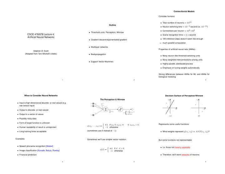
Decision Surface of Perceptron/Winnow The Perceptron & Winnow x2 x2 + • Input is high-dimensional discrete- or real-valued (e.g. + x 1 w 1 x 0 =1 - - + w 0 raw sensor input) x 2 w 2 + . � x1 x1 • Output is discrete- or real-valued . n n - � wi xi { - + . � wi xi 1 if > 0 - i =0 o = w n i =0 • Output is a vector of values -1 otherwise x n ( a ) ( b ) • Possibly noisy data • Form of target function is unknown ( Represents some useful functions +1 if w 0 + w 1 x 1 + · · · + w n x n > 0 o ( x 1 , . . . , x n ) = • Human readability of result is unimportant � 1 otherwise (sometimes use 0 instead of � 1 ) • Long training times acceptable • What weights represent g ( x 1 , x 2 ) = AND ( x 1 , x 2 ) ? Examples: Sometimes we’ll use simpler vector notation: But some functions not representable • Speech phoneme recognition [Waibel] • I.e. those not linearly separable ( +1 if ~ w · ~ x > 0 o ( ~ x ) = • Image classification [Kanade, Baluja, Rowley] � 1 otherwise • Therefore, we’ll want networks of neurons • Financial prediction 4 5 6

  2. Perceptron vs. Winnow Winnow works well when most attributes irrelevant, i.e. Winnow Training Rule w ⇤ is sparse (many 0 entries) when optimal weight vector ~ Perceptron Training Rule x 2 { 0 , 1 } n be labeled by a E.g. let examples ~ k -disjunction over n attributes, k ⌧ n w i w i · ∆ w mult , where ∆ w mult = ↵ ( t � o ) x i i i • Remaining n � k are irrelevant w i w i + ∆ w add , where ∆ w add = ⌘ ( t � o ) x i and ↵ > 1 i i • E.g. c ( x 1 , . . . , x 150 ) = x 5 _ x 9 _ ¬ x 12 , n = 150 , and I.e. use multiplicative updates vs. additive updates k = 3 • t = c ( ~ x ) is target value • For disjunctions, number of prediction mistakes (in on- Problem: Sometimes negative weights are required • o is perceptron output line model) is O ( k log n ) for Winnow and (in worst case) Ω ( kn ) for Perceptron w + and ~ w � and replace • Maintain two weight vectors ~ • ⌘ is small constant (e.g. 0.1) called learning rate ⇣ w � ⌘ w + � ~ w · ~ ~ x with ~ · ~ x • So in worst case, need exponentially fewer updates I.e. if ( t � o ) > 0 then increase w i w.r.t. x i , else decrease w + and ~ w � independently as above, using for learning with Winnow than Perceptron • Update ~ ∆ w + = ↵ ( t � o ) x i and ∆ w � i = 1 / ∆ w + i i Can prove rule will converge if training data is linearly sep- Bound is only for disjunctions, but improvement for learn- arable and ⌘ sufficiently small ing with irrelevant attributes is often true Can also guarantee convergence w ⇤ not sparse, sometimes Perceptron better When ~ Also, have proofs for agnostic error bounds for both algo- rithms 7 8 9 Gradient Descent and Exponentiated Gradient Gradient Descent • Useful when linear separability impossible but still want to minimize training error Gradient Descent and Exponentiated Gradient conserv. corrective coef. (cont’d) z }| { z }| { • Consider simpler linear unit , where w d k 2 x d ) 2 z}|{ U ( ~ w ) = k ~ w d +1 � ~ 2 + ( t d � ~ w d +1 · ~ ⌘ 25 2 0 1 o = w 0 + w 1 x 1 + · · · + w n x n n n ⌘ 2 + ⌘ ⇣ X X 20 = w i,d +1 � w i,d @ t d � w i,d +1 x i,d A (i.e. no threshold) i =1 i =1 15 E[w] • For moment, assume that we update weights after 10 w d +1 and set to ~ seeing each example ~ x d 0 : Take gradient w.r.t. ~ 5 0 1 n • For each example, want to compromise between ⇣ ⌘ X A x i,d 0 = 2 � 2 ⌘ w i,d +1 � w i,d @ t d � w i,d +1 x i,d 0 correctiveness and conservativeness 2 i =1 1 -2 – Correctiveness: Tendency to improve on ~ x d (re- -1 0 0 Approximate with duce error) 1 0 1 n 2 -1 ⇣ ⌘ 3 X A x i,d , 0 = 2 w i,d +1 � w i,d � 2 ⌘ @ t d � w i,d x i,d w1 w0 – Conservativeness: Tendency to keep i =1 w d +1 close to ~ ~ w d (minimize distance) " # @ U @ U , @ U , · · · , @ U w = which yields @ ~ @ w 0 @ w 1 @ w n • Use cost function that measures both: ∆ w add i,d z }| { w i,d +1 = w i,d + ⌘ ( t d � o d ) x i,d 0 1 curr ex, new wts ⇣ ⌘ z }| { U ( ~ w ) = dist w d +1 , ~ ~ w d + ⌘ error @ t d , w d +1 · ~ ~ x d A 10 11 12

  3. Remarks Implementation Approaches Exponentiated Gradient • Perceptron and Winnow update weights based on thresh- olded output, while GD and EG use unthresholded outputs Conserv. portion uses unnormalized relative entropy: • Can use rules on previous slides on an example-by- conserv. example basis, sometimes called incremental, stochastic, corrective z }| { n coef. ✓ ◆ • P/W converge in finite number of steps to perfect hyp X w i,d � w i,d +1 + w i,d +1 ln w i,d +1 z }| { or on-line GD/EG z}|{ x d ) 2 U ( ~ w ) = + ⌘ ( t d � ~ w d +1 · ~ if data linearly separable; GD/EG work on non-linearly w i,d i =1 separable data, but only converge asymptotically (to – Has a tendency to “jump around” more in search- wts with minimum squared error) ing, which helps avoid getting trapped in local min- w d +1 and set to ~ Take gradient w.r.t. ~ 0 : ima 0 1 n 0 = ln w i,d +1 X • As with P vs. W, EG tends to work better than GD A x i,d � 2 ⌘ @ t d � w i,d +1 x i,d w i,d when many attributes are irrelevant i =1 • Alternatively, can use standard or batch GD/EG, in – Allows the addition of attributes that are nonlinear which the classifier is evaluated over all training exam- Approximate with combinations of original ones, to work around lin- 0 1 ples, summing the error, and then updates are made n 0 = ln w i,d +1 X ear sep. problem (perhaps get linear separability A x i,d , � 2 ⌘ @ t d � w i,d x i,d w i,d in new, higher-dimensional space) i =1 – I.e. sum up ∆ w i for all examples, but don’t update w i until summation complete (p. 93, Table 4.1) – E.g. if two attributes are x 1 and x 2 , use as EG which yields (for ⌘ = ln ↵ / 2 ) ∆ w mult inputs i,d – This is an inherent averaging process and tends to z }| { h i ⇣ ⌘ ↵ ( t d � o d ) x i,d x 1 , x 2 , x 1 x 2 , x 2 1 , x 2 = w i,d exp 2 ⌘ ( t d � o d ) x i,d = w i,d ~ x = w i,d +1 give better estimate of the gradient 2 • Also, both have provable agnostic results 13 14 15 The XOR Problem The XOR Problem Handling Nonlinearly Separable Data x (cont’d) (cont’d) The XOR Problem 2 8 • In other words, we remapped all vectors ~ x to ~ y such < 0 if g i ( ~ x ) < 0 • Let y i = D: (1,1) that the classes are linearly separable in the new vec- 1 otherwise : tor space B: (0,1) neg w = -1/2 Class ( x 1 , x 2 ) g 1 ( ~ x ) y 1 g 2 ( ~ x ) y 2 Hidden Layer 30 y 1 B: (0 , 1) 1 / 2 1 � 1 / 2 pos 0 pos g (x) pos C: (1 , 0) 1 / 2 1 � 1 / 2 0 w = -1/2 2 50 w = 1 � neg > 0 neg A: (0 , 0) � 1 / 2 0 � 3 / 2 0 w x 31 w = 1 3i i i 53 < 0 neg D: (1 , 1) 3 / 2 1 1 / 2 1 x 1 x Input Layer w = 1 � w y 32 1 5i i A: (0,0) C: (1,0) i > 0 x w = 1 • Now feed y 1 , y 2 into: 2 41 < 0 g (x) 1 w = -2 w = 1 � Output g ( ~ y ) = 1 · y 1 � 2 · y 2 � 1 / 2 w x i 54 42 4i y i 2 Layer g(y) y 2 < 0 D: (1,1) • Can’t represent with a single linear separator, but can w = -3/2 > 0 40 with intersection of two: neg g 1 ( ~ x ) = 1 · x 1 + 1 · x 2 � 1 / 2 pos • This is a two-layer perceptron or two-layer g 2 ( ~ x ) = 1 · x 1 + 1 · x 2 � 3 / 2 feedforward neural network n o x 2 R ` : g 1 ( ~ pos = ~ x ) > 0 AND g 2 ( ~ x ) < 0 y 1 A: (0,0) B, C: (1,0) • Each neuron outputs 1 if its weighted sum exceeds its n o x 2 R ` : g 1 ( ~ threshold, 0 otherwise neg = ~ x ) , g 2 ( ~ x ) < 0 OR g 1 ( ~ x ) , g 2 ( ~ x ) > 0 16 17 18

Download Presentation
Download Policy: The content available on the website is offered to you 'AS IS' for your personal information and use only. It cannot be commercialized, licensed, or distributed on other websites without prior consent from the author. To download a presentation, simply click this link. If you encounter any difficulties during the download process, it's possible that the publisher has removed the file from their server.

Recommend


More recommend