why quantum wave probability
play

Why Quantum (Wave Probability) Need for a Geometric . . . Models - PowerPoint PPT Presentation

Quantum Models Are . . . Ubiquity of Multi-D . . . Let Us Simplify the . . . For Complex Systems, . . . Why Quantum (Wave Probability) Need for a Geometric . . . Models Are a Good Description of Many Geometric Description . . . Non-Quantum


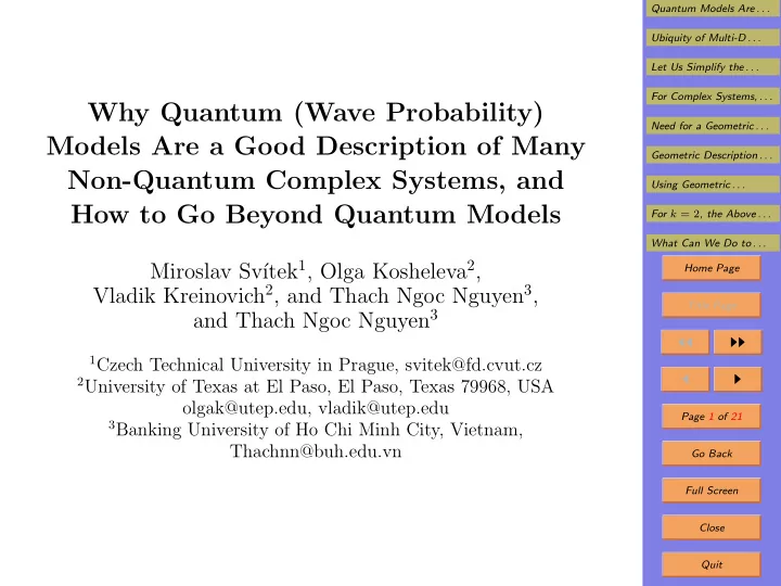
  1. Quantum Models Are . . . Ubiquity of Multi-D . . . Let Us Simplify the . . . For Complex Systems, . . . Why Quantum (Wave Probability) Need for a Geometric . . . Models Are a Good Description of Many Geometric Description . . . Non-Quantum Complex Systems, and Using Geometric . . . How to Go Beyond Quantum Models For k = 2 , the Above . . . What Can We Do to . . . ıtek 1 , Olga Kosheleva 2 , Miroslav Sv´ Home Page Vladik Kreinovich 2 , and Thach Ngoc Nguyen 3 , Title Page and Thach Ngoc Nguyen 3 ◭◭ ◮◮ 1 Czech Technical University in Prague, svitek@fd.cvut.cz ◭ ◮ 2 University of Texas at El Paso, El Paso, Texas 79968, USA olgak@utep.edu, vladik@utep.edu Page 1 of 21 3 Banking University of Ho Chi Minh City, Vietnam, Thachnn@buh.edu.vn Go Back Full Screen Close Quit
  2. Quantum Models Are . . . Ubiquity of Multi-D . . . 1. Quantum Models Are Often a Good Descrip- Let Us Simplify the . . . tion of Non-Quantum Systems For Complex Systems, . . . • Quantum physics has been designed to describe quan- Need for a Geometric . . . tum objects. Geometric Description . . . Using Geometric . . . • These are objects – mostly microscopic but sometimes For k = 2 , the Above . . . macroscopic as well – that exhibit quantum behavior. What Can We Do to . . . • Somewhat surprisingly, however, it turns out that quantum- Home Page type techniques can also be useful in describing non- Title Page quantum complex systems. ◭◭ ◮◮ • For example, they describe economic systems and other ◭ ◮ systems involving human behavior. Page 2 of 21 • Why quantum techniques can help in non-quantum sit- uations is largely a mystery. Go Back Full Screen Close Quit

  3. Quantum Models Are . . . Ubiquity of Multi-D . . . 2. Quantum Models (cont-d) Let Us Simplify the . . . • The next natural question is related to the fact that: For Complex Systems, . . . Need for a Geometric . . . – while quantum models provide a good description Geometric Description . . . of non-quantum systems, Using Geometric . . . – this description is not perfect. For k = 2 , the Above . . . • So, a natural question: how to get a better approxima- What Can We Do to . . . tion? Home Page • In this talk, we provide answers to the above two ques- Title Page tions. ◭◭ ◮◮ ◭ ◮ Page 3 of 21 Go Back Full Screen Close Quit

  4. Quantum Models Are . . . Ubiquity of Multi-D . . . 3. Ubiquity of Multi-D Normal Distributions Let Us Simplify the . . . • To describe the state of a complex system, we need to For Complex Systems, . . . describe the values of some quantities x 1 , . . . , x n . Need for a Geometric . . . Geometric Description . . . • In many cases, the system consists of a large number Using Geometric . . . of reasonably independent parts; in this case: For k = 2 , the Above . . . – each of the quantities x i describing the system What Can We Do to . . . – is approximately equal to the sum of the values that Home Page describes these parts. Title Page • E.g., the country’s trade volume is the sum of the ◭◭ ◮◮ trades performed by all its companies. ◭ ◮ • The number of country’s unemployed people is the sum Page 4 of 21 of numbers from different regions, etc. Go Back Full Screen Close Quit

  5. Quantum Models Are . . . Ubiquity of Multi-D . . . 4. Multi-D Normal Distributions (cont-d) Let Us Simplify the . . . • It is known that: For Complex Systems, . . . Need for a Geometric . . . – the distribution of the sum of a large number of Geometric Description . . . independent random variables Using Geometric . . . – is – under certain reasonable conditions – close to For k = 2 , the Above . . . Gaussian (normal). What Can We Do to . . . • This result is known as the Central Limit Theorem . Home Page • Thus, with reasonable accuracy, we can assume that: Title Page ◭◭ ◮◮ – the vectors x = ( x 1 , . . . , x n ) formed by all the quan- tities that characterize the system as a whole ◭ ◮ – are normally distributed. Page 5 of 21 Go Back Full Screen Close Quit

  6. Quantum Models Are . . . Ubiquity of Multi-D . . . 5. Let Us Simplify the Description of the Multi-D Let Us Simplify the . . . Normal Distribution For Complex Systems, . . . • A multi-D normal distr. is uniquely characterized: Need for a Geometric . . . Geometric Description . . . def – by its means µ = ( µ 1 , . . . , µ n ), µ i = E [ x i ], and Using Geometric . . . def – by its covariance matrix σ ij = E [( x i − µ i ) · ( x j − µ j )]. For k = 2 , the Above . . . • By observing the values x i corresponding to different What Can We Do to . . . Home Page systems, we can estimate the mean values µ i . Title Page • Instead of the original values x i , we can consider devi- def ◭◭ ◮◮ ations δ i = x i − µ i ; then, E [ δ i ] = 0, so: ◭ ◮ – to fully describe the distribution of the correspond- ing vector δ = ( δ 1 , . . . , δ n ), Page 6 of 21 – it is sufficient to know the covariance matrix σ ij . Go Back • Since E [ δ i ] = 0, we have σ ij = E [ δ i · δ j ]. Full Screen Close Quit

  7. Quantum Models Are . . . Ubiquity of Multi-D . . . 6. For Complex Systems, with a Large Number of Let Us Simplify the . . . Parameters, a Further Simplification Is Needed For Complex Systems, . . . • To fully describe the distribution, we need to describe Need for a Geometric . . . all the values of the n × n covariance matrix σ ij . Geometric Description . . . • In general, an n × n matrix contains n 2 elements. Using Geometric . . . For k = 2 , the Above . . . • Ssince the covariance matrix is symmetric, we only What Can We Do to . . . = n 2 need to describe n · ( n + 1) 2 + n 2 parameters. Home Page 2 • Can we determine all these parameters from the obser- Title Page vations? In general in statistics: ◭◭ ◮◮ – if we want to find a reasonable estimate for a pa- ◭ ◮ rameter, Page 7 of 21 – we need to have a certain number of observations. Go Back • Based on N observations, we can find the value of each 1 Full Screen √ quantity with accuracy ≈ . N Close Quit

  8. Quantum Models Are . . . Ubiquity of Multi-D . . . 7. Simplification Is Needed (cont-d) Let Us Simplify the . . . • Thus, to be able to determine a parameter with a rea- For Complex Systems, . . . sonable accuracy of 20%, we need to select N for which Need for a Geometric . . . Geometric Description . . . 1 √ ≈ 20% = 0 . 2 , i.e., N = 25 . Using Geometric . . . N For k = 2 , the Above . . . • So, to find the value of one parameter, we need approx- What Can We Do to . . . imately 25 observations. Home Page • By the same logic, for any integer k , to find the values Title Page of k parameters, we need to have 25 k observations. ◭◭ ◮◮ ≈ n 2 • In particular, to determine n · ( n + 1) ◭ ◮ 2 parame- 2 ters, we need to have 25 · n 2 Page 8 of 21 2 observations. Go Back • Each fully detailed observation of a system leads to n Full Screen numbers x 1 , . . . , x n and thus, to n numbers δ 1 , . . . , δ n . Close Quit

  9. Quantum Models Are . . . Ubiquity of Multi-D . . . 8. Simplification Is Needed (cont-d) Let Us Simplify the . . . • So, to estimate 25 · n 2 For Complex Systems, . . . 2 = 12 . 5 · n 2 parameters, we need Need for a Geometric . . . to have 12 . 5 · n different systems. Geometric Description . . . • And we often do not have that many system to observe. Using Geometric . . . For k = 2 , the Above . . . • For example, for a detailed analysis of a country’s econ- What Can We Do to . . . omy, we need to have n ≥ 30 parameters. Home Page • To fully describe the joint distribution of all these pa- Title Page rameters, we need ≥ 12 . 5 · 30 ≈ 375 countries. ◭◭ ◮◮ • We do not have that many countries. ◭ ◮ • This problem occurs not only in econometrics, it is even Page 9 of 21 more serious, e.g., in medical bioinformatics. Go Back • There are thousands of genes, and not enough data to Full Screen be able to determine all the correlations between them. Close Quit

  10. Quantum Models Are . . . Ubiquity of Multi-D . . . 9. Simplification Is Needed (cont-d) Let Us Simplify the . . . • So we cannot determine the covariance matrix σ ij ex- For Complex Systems, . . . actly. Need for a Geometric . . . Geometric Description . . . • Thus, we need to come up with an approximate de- Using Geometric . . . scription, with fewer parameters. For k = 2 , the Above . . . What Can We Do to . . . Home Page Title Page ◭◭ ◮◮ ◭ ◮ Page 10 of 21 Go Back Full Screen Close Quit

  11. Quantum Models Are . . . Ubiquity of Multi-D . . . 10. Need for a Geometric Description Let Us Simplify the . . . • What does it means to have a good approximation? For Complex Systems, . . . Need for a Geometric . . . • Intuitively, approximations means having a model which Geometric Description . . . is, in some reasonable sense, close to the original one. Using Geometric . . . • In other words, we need model whose distance from the For k = 2 , the Above . . . original model is small. What Can We Do to . . . Home Page • So, we need to represent objects by points in a metric space. Title Page • So, it is desirable to use an appropriate geometric rep- ◭◭ ◮◮ resentation of multi-D normal distributions. ◭ ◮ • Such a representation is well known. Page 11 of 21 Go Back Full Screen Close Quit

Download Presentation
Download Policy: The content available on the website is offered to you 'AS IS' for your personal information and use only. It cannot be commercialized, licensed, or distributed on other websites without prior consent from the author. To download a presentation, simply click this link. If you encounter any difficulties during the download process, it's possible that the publisher has removed the file from their server.

Recommend


More recommend