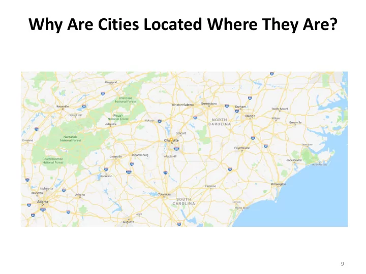
Why Are Cities Located Where They Are? 9 Taxonomy of Location - PowerPoint PPT Presentation

Why Are Cities Located Where They Are? 9

Taxonomy of Location Problems Location Decision Cooperative Competitive Minimize System Costs Minimize Individual Costs Location Location Minimize Sum of Costs Minimax Cost “Nonlinear” Minisum Location Maximin Cost Location Sum of Costs = SC = TC + LC Center of Gravity LC > TC TC > LC Transport Oriented Local-Input Oriented Local Input Costs = LC = labor Location Location Transport Costs = TC = PC + DC costs, ubiquitous input costs, etc. PC > DC DC > PC Resource Oriented Market Oriented Procurement Costs = PC Distribution Costs = DC Location Location “Weight - losing” activities “Weight - gaining” activities 10

Hotelling's Law 34 0 1 34 0 1 1 2 0 1 1 4 34 0 1 11

1-D Cooperative Location Durham Raleigh US-70 (Glenwood Ave.) 1 2 0 30 w 1 = 1 w 2 = 2     a 0, a 30 Min TC w d 1 2 i i     2    2 TC w d w x a   i i i i 2 Min TC w d i i dTC        2 0 w x a i i   dx k Min TC w d i i     x w w a i i i   w a 1(0) 2(30) i i Squared−Euclidean Distance  Center of Gravity :    * 20 x   1 2 w i 12

“Nonlinear” Location   k TC w d i i 13

Minimax and Maximin Location • Minimax – Min max distance – Set covering problem • Maximin – Max min distance – AKA obnoxious facility location 14

2-EF Minisum Location +w 1 +w 2 TC +8 -w 1 -w 2 +w 1 -8 90 w - w 2 + 1 -w 2 +2 -3 -w 1 +w 2 -5 +5 +3 2 1 x 10 25 30   , if  w x x           i i ( ) ( ) ( ), where TC x w d x x x x 1 1 2 2  i i i  , if w x x i i      (25) (25 10) ( )(25 30) TC w w 1 2      5(15) ( 3)( 5) 90 15

Median Location: 1-D 4 EFs TC Minimum at point where TC curve slope switches from (-) to (+) +14 -14 +6 -4 +2 1 2 3 4 w i 5 3 2 4 -5-3-2-4 = -14 +5-3-2-4 = -4 +5+3-2-4 = +2 +5+3+2-4 = +6 +5+3+2+4 = +14 5 < W/2 5+3=8 > W/2 4+2+3=9 > W/2 4+2=6 < W/2 4 < W/2 16

Median Location: 1-D 7 EFs 36.5 Winston-Salem Greensboro Durham 190 36 220 Raleigh 270 Statesville 295 Asheville 150 35.5 50 40 35 Wilmington 34.5 420 34 -83 -82 -81 -80 -79 -78 w : 6 4 3 2 1 3 5 i j W 6<12 10<12 13>12   : w 14>12 11<12 9<12 8<12 5<12 i 2  1 i * 17

Median Location: 2-D Rectilinear Distance 8 EFs w i : y : 62 < 129     ( , ) d P P x x y y 1 1 2 1 2 1 2 9 53 62 95 5 2     2 2     ( , ) d P P x x y y 2 1 2 1 2 1 2 81 < 129 19 19 70 1 42 6 * 129 = 129 48 60 4 8 Y Optimal location 129 = 129 anywhere along line 82 8 90 25 3 6 * 39 39 < 129 39 15 7 : x 5 15 60 70 90 X : w i 101 50 48 53 6 101 < 129 151 > 129 157 > 129 107 < 129 59 < 129 6 < 129 18 *

Ex 3: 2D Loc with Rect Approx to GC Dist • It is expected that 25, 42, 24, 10, 24, and 11 truckloads will be shipped each year from your DC to six customers located in Raleigh, NC (36N,79W), Atlanta, GA (34N,84W), Louisville, KY (38N,86W), Greenville, SC (35N, 82W), Richmond, VA (38N,77W), and Savannah, GA (32N,81W). Assuming that all distances are rectilinear, where should the DC be located in order to minimize outbound transportation costs? 24 24 48 * 88<68 25 25 10 63<68 10 42 42 53<68 11 11<68 11 W     136, 68 W w i 2 24 42 10 11 25 24 Optimal location (36N,82W) Answer : 24<68 66<68 76>68 * (65 mi from opt great-circle location) 19

Logistics Network for a Plant Customers Tier Two Suppliers Tier One Plant DCs Suppliers D D D D A BBBB EEEE A B = D + E A A Resource Market A CCCC A A = B + C FFFF A GGGG A C = F + G downstream upstream Assembly Network vs. Distribution Network Procurement vs. Distribution Inbound Logistics vs. Outbound Logistics Raw Materials vs. Finished Goods 20

Basic Production System ubiquitous inputs 1 ton raw finished material goods Production Supplier Customer System 4 ton 3 ton 2 ton scrap title transfer title transfer FOB Origin FOB Destination you pay you pay Seller Buyer Seller Buyer FOB Destination FOB Origin supplier pays customer pays title transfer title transfer Inbound Outbound FOB (free on board) 21

FOB and Location • Choice of FOB terms (who directly pays for transport) usually does not impact location decisions: Procurement Landed cost Inbound transport   cost cost at supplier Production Procurement Local resource   cost cost cost (labor, etc.) Total delivered Production Outbound transport   cost cost co s t Transport cos t Inbound transport Outbound transport   (T C) cost cost – Purchase price from supplier and sale price to customer adjusted to reflect who is paying transport cost – Usually determined by who can provide the transport at the lowest cost • Savings in lower transport cost allocated (bargained) between parties 22

Monetary vs. Physical Weight m m     min TC X ( ) w d X P ( , ) f r d X P ( , ) i i i i i   1 1 i i w i  where total transport cost ($/yr) TC  monetary weight ($/mi-yr) w i  physical weight rate (ton/yr) f i  transport rate ($/ton-mi) r i  ( , ) distance between NF at an d EF at (mi) d X P X P i i i NF = new facility to be located EF = existing facility m  number of EFs    (Montetary) Weight Gaining: w w in out    Physically Weight Losing: f f in out 23

Minisum Location: TC vs. TD • Assuming local input costs are – same at every location or – insignificant as compared to transport costs, the minisum transport-oriented single-facility location problem is to locate NF to minimize TC • Can minimize total distance (TD) if transport rate is same: m m     min ( ) ( , ) ( , ) TD X w d X P f r d X P i i i i i   1 1 i i w i  where total transport distance (mi/yr) TD  monetary weight (trip/yr) w i  trips per year (trip/ yr) f i  transport rate = 1 r i  ( , ) per-trip distance between NF an E d F (mi/trip) d X P i i 24

Ex 4: Single Supplier and Customer Location 36.5 raw finished Winston-Salem material goods Greensboro Asheville Product A Durham Durham 36 190 220 2 ton 1 ton 270 Raleigh Statesville 295 Asheville 150 1 ton 35.5 50 scrap 40 35 ubiquitous Wilmington inputs 34.5 2 ton raw finished 420 material goods Winston- 34 Wilmington Product B Salem 1 ton 3 ton -83 -82 -81 -80 -79 -78 • The cost per ton-mile (i.e., the cost to ship one ton, one mile) for both raw materials and finished goods is the same (e.g., $0.10). 1. Where should the plant for each product be located? 2. How would location decision change if customers paid for distribution costs (FOB Origin) instead of the producer (FOB Destination)? • In particular, what would be the impact if there were competitors located along I-40 producing the same product? 3. Which product is weight gaining and which is weight losing? 4. If both products were produced in a single m   ( ) ( , ) TC X f r d X P shared plant, why is it now necessary to i i i  i 1 w know each product’s annual demand ( f i )? i 25

Ex 5: 1-D Location with Procurement and Distribution Costs unit of Asheville finished good Production System 1 ton Durham Assume: all scrap is disposed of locally A product is to be produced in a plant that will be located along I-40. Two tons of raw materials from a supplier in Ashville and a half ton of a raw material from a supplier in Durham are used to produce each ton of finished product that is shipped to customers in Statesville, Winston-Salem, and Wilmington. The demand of these customers is 10, 20, and 30 tons, respectively, and it costs $0.33 per ton-mile to ship raw materials to the plant and $1.00 per ton-mile to ship finished goods from the plant. Determine where the plant should be located so that procurement and distribution costs (i.e., transportation costs to and from the plant) are minimized, and whether the plant is weight gaining or weight losing. 26