What is Statistical Learning? 25 25 25 20 20 20 Sales 15 - - PowerPoint PPT Presentation

What is Statistical Learning?

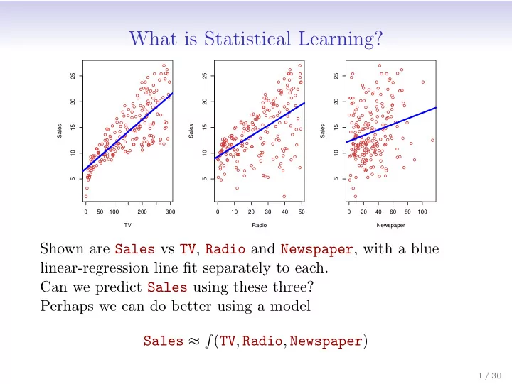
50 100 200 300 5 10 15 20 25 TV Sales 10 20 30 40 50 5 10 15 20 25 Radio Sales 20 40 60 80 100 5 10 15 20 25 Newspaper Sales

Shown are Sales vs TV, Radio and Newspaper, with a blue linear-regression line fit separately to each. Can we predict Sales using these three? Perhaps we can do better using a model Sales ≈ f(TV, Radio, Newspaper)

1 / 30

Notation

Here Sales is a response or target that we wish to predict. We generically refer to the response as Y . TV is a feature, or input, or predictor; we name it X1. Likewise name Radio as X2, and so on. We can refer to the input vector collectively as X =    X1 X2 X3    Now we write our model as Y = f(X) + ǫ where ǫ captures measurement errors and other discrepancies.

2 / 30

What is f(X) good for?

• With a good f we can make predictions of Y at new points

X = x.

• We can understand which components of

X = (X1, X2, . . . , Xp) are important in explaining Y , and which are irrelevant. e.g. Seniority and Years of Education have a big impact on Income, but Marital Status typically does not.

• Depending on the complexity of f, we may be able to

understand how each component Xj of X affects Y .

3 / 30

• ●
• ●
• ●
• ●
• ●
• ●
• ●
• ●
• ●
• ●
• ●
• ●
• ●
• ●
• ●
• ●
• ●
• ●
• 1

2 3 4 5 6 7 −2 2 4 6 x y

• Is there an ideal f(X)? In particular, what is a good value for

f(X) at any selected value of X, say X = 4? There can be many Y values at X = 4. A good value is f(4) = E(Y |X = 4) E(Y |X = 4) means expected value (average) of Y given X = 4. This ideal f(x) = E(Y |X = x) is called the regression function.

4 / 30

The regression function f(x)

• Is also defined for vector X; e.g.

f(x) = f(x1, x2, x3) = E(Y |X1 = x1, X2 = x2, X3 = x3)

• Is the ideal or optimal predictor of Y with regard to

mean-squared prediction error: f(x) = E(Y |X = x) is the function that minimizes E[(Y − g(X))2|X = x] over all functions g at all points X = x.

• ǫ = Y − f(x) is the irreducible error — i.e. even if we knew

f(x), we would still make errors in prediction, since at each X = x there is typically a distribution of possible Y values.

• For any estimate ˆ

f(x) of f(x), we have E[(Y − ˆ f(X))2|X = x] = [f(x) − ˆ f(x)]2

• Reducible

+ Var(ǫ)

Irreducible

5 / 30

How to estimate f

• Typically we have few if any data points with X = 4

exactly.

• So we cannot compute E(Y |X = x)!
• Relax the definition and let

ˆ f(x) = Ave(Y |X ∈ N(x)) where N(x) is some neighborhood of x.

• 1

2 3 4 5 6 −2 −1 1 2 3 x y

• 6 / 30

• Nearest neighbor averaging can be pretty good for small p

— i.e. p ≤ 4 and large-ish N.

• We will discuss smoother versions, such as kernel and

spline smoothing later in the course.

• Nearest neighbor methods can be lousy when p is large.

Reason: the curse of dimensionality. Nearest neighbors tend to be far away in high dimensions.

• We need to get a reasonable fraction of the N values of yi

to average to bring the variance down—e.g. 10%.

• A 10% neighborhood in high dimensions need no longer be

local, so we lose the spirit of estimating E(Y |X = x) by local averaging.

7 / 30

The curse of dimensionality

• ●
• −1.0

−0.5 0.0 0.5 1.0 −1.0 −0.5 0.0 0.5 1.0 x1 x2

10% Neighborhood

• 0.0

0.1 0.2 0.3 0.4 0.5 0.6 0.7 0.0 0.5 1.0 1.5 Fraction of Volume Radius p= 1 p= 2 p= 3 p= 5 p= 10

8 / 30

Parametric and structured models

The linear model is an important example of a parametric model: fL(X) = β0 + β1X1 + β2X2 + . . . βpXp.

• A linear model is specified in terms of p + 1 parameters

β0, β1, . . . , βp.

• We estimate the parameters by fitting the model to

training data.

• Although it is almost never correct, a linear model often

serves as a good and interpretable approximation to the unknown true function f(X).

9 / 30

A linear model ˆ fL(X) = ˆ β0 + ˆ β1X gives a reasonable fit here

• 1

2 3 4 5 6 −2 −1 1 2 3 x y

• A quadratic model ˆ

fQ(X) = ˆ β0 + ˆ β1X + ˆ β2X2 fits slightly better.

• 1

2 3 4 5 6 −2 −1 1 2 3 x y

• 10 / 30

Y e a r s

• f

E d u c a t i

• n

Seniority I n c

• m

e

Simulated example. Red points are simulated values for income from the model income = f(education, seniority) + ǫ f is the blue surface.

11 / 30

Y e a r s

• f

E d u c a t i

• n

Seniority I n c

• m

e

Linear regression model fit to the simulated data. ˆ fL(education, seniority) = ˆ β0+ˆ β1×education+ˆ β2×seniority

12 / 30

Y e a r s

• f

E d u c a t i

• n

Seniority I n c

• m

e

More flexible regression model ˆ fS(education, seniority) fit to the simulated data. Here we use a technique called a thin-plate spline to fit a flexible surface. We control the roughness of the fit (chapter 7).

13 / 30

Y e a r s

• f

E d u c a t i

• n

Seniority I n c

• m

e

Even more flexible spline regression model ˆ fS(education, seniority) fit to the simulated data. Here the fitted model makes no errors on the training data! Also known as overfitting.

14 / 30

Some trade-offs

• Prediction accuracy versus interpretability.

— Linear models are easy to interpret; thin-plate splines are not.

• Good fit versus over-fit or under-fit.

— How do we know when the fit is just right?

• Parsimony versus black-box.

— We often prefer a simpler model involving fewer variables over a black-box predictor involving them all.

15 / 30

Flexibility Interpretability

Low High Low High

Subset Selection Lasso Least Squares Generalized Additive Models Trees Bagging, Boosting Support Vector Machines

16 / 30

Assessing Model Accuracy

Suppose we fit a model ˆ f(x) to some training data Tr = {xi, yi}N

1 , and we wish to see how well it performs.

• We could compute the average squared prediction error
• ver Tr:

MSETr = Avei∈Tr[yi − ˆ f(xi)]2 This may be biased toward more overfit models.

• Instead we should, if possible, compute it using fresh test

data Te = {xi, yi}M

1 :

MSETe = Avei∈Te[yi − ˆ f(xi)]2

17 / 30

20 40 60 80 100 2 4 6 8 10 12 X Y 2 5 10 20 0.0 0.5 1.0 1.5 2.0 2.5 Flexibility Mean Squared Error

Black curve is truth. Red curve on right is MSETe, grey curve is

• MSETr. Orange, blue and green curves/squares correspond to fits of

different flexibility.

18 / 30

20 40 60 80 100 2 4 6 8 10 12 X Y 2 5 10 20 0.0 0.5 1.0 1.5 2.0 2.5 Flexibility Mean Squared Error

Here the truth is smoother, so the smoother fit and linear model do really well.

19 / 30

20 40 60 80 100 −10 10 20 X Y 2 5 10 20 5 10 15 20 Flexibility Mean Squared Error

Here the truth is wiggly and the noise is low, so the more flexible fits do the best.

20 / 30

Bias-Variance Trade-off

Suppose we have fit a model ˆ f(x) to some training data Tr, and let (x0, y0) be a test observation drawn from the population. If the true model is Y = f(X) + ǫ (with f(x) = E(Y |X = x)), then E

• y0 − ˆ

f(x0) 2 = Var( ˆ f(x0)) + [Bias( ˆ f(x0))]2 + Var(ǫ). The expectation averages over the variability of y0 as well as the variability in Tr. Note that Bias( ˆ f(x0))] = E[ ˆ f(x0)] − f(x0). Typically as the flexibility of ˆ f increases, its variance increases, and its bias decreases. So choosing the flexibility based on average test error amounts to a bias-variance trade-off.

21 / 30

Bias-variance trade-off for the three examples

2 5 10 20 0.0 0.5 1.0 1.5 2.0 2.5 Flexibility 2 5 10 20 0.0 0.5 1.0 1.5 2.0 2.5 Flexibility 2 5 10 20 5 10 15 20 Flexibility MSE Bias Var

22 / 30

Classification Problems

Here the response variable Y is qualitative — e.g. email is one

• f C = (spam, ham) (ham=good email), digit class is one of

C = {0, 1, . . . , 9}. Our goals are to:

• Build a classifier C(X) that assigns a class label from C to

a future unlabeled observation X.

• Assess the uncertainty in each classification
• Understand the roles of the different predictors among

X = (X1, X2, . . . , Xp).

23 / 30

| | | | | | | | | | | | | | | | | | | | | | | | | | | | || | | | | | | | | | || | | | | | | | | | | | | | | | | || | | | | | | | | | | | | | | | | | | | | | | | | | | | | | | | | | | | | | | | | | | | | | | | | | | | | | | | | | | | | | | | | | | | | | | | | | | | | | | | | | | | | | | | | | | | | | | | | | | | | | | | | | | | | | | | | | | | | | | | | | | | | | | | | | | | | | | | | | | | | | | | | | | | | | | | | | | | | | | | | | | | | | | | | | | | | | | | | | | | | | | | | | | | | | | | | | | | | | | | | | | | | | | | | | | | | | | | | | | | | | | | | | | | | | | | | | | | | | | | || | | | | | | | | | | | | | | | | | | | | | | | | | | | | | | | | | | | | | | | | | | | | | | | | | | | | | | | | | | | | | | | | | | | | | | | | | | | | | | | | | | | | | | | | | | | | | | | | | | | | | | | | | | | | | | | | | | | | | | | | | | | | | | | | | | | | | | | | | | | | | | | | | | | | | | | | | | | | | | | | | | | | | | | | | | | | | | | | | | | | | | | | | | | | | | | | | | | | | | | | | | | | | | | | | | | | | | | | | | | | | | | | | | | | | | | | | | | | | | | | | | | | | | | | | | | | | | | | | | | | | | | | | | | | | | | | | | | | || | | | | | | | | | | | | | | | | | | | | | | | | | | | | | | | | | | | | | | | | | | | | | | | | | ||| ||| | | | | | | | | | | | | | | | | | | | | | | | | | | | | | | | | | | | | | | | | | | | | | | | | | | | | | | | | | | | | | | | | | | | | | | | | | | | | | | | | | | | | | | | | | | | | | | | | | | | | | | | | | | | | | | | | | | | | | | | | | | | | | | | | | | | | | | | | | | | | | | | | | | | | | | | | | | | | | | | | | | || | | | | | | | | | | | | | | | | | | | | | | | | | | | | | | | | | | | | | | | | | | | | | | | | | | | | | | | | | | | | | | | | | | | | | | | | | | | | | | | | | | | | | | | | | | | | | | | | | | | | | | | | | | | | | | | | | | | | | | | | | | | | | | | | | | | | | | | | | | | | | | | | | | | | | | | | | | | | | | | | | | | | | | | | | | | | | | | | | | | | | | | | | | | | | | | | | | | | | | | | | | | | | | | | | | | | | | | | | | | | | | | | | | | | | | | | | | | | | | | | | | | | | | | | | | | | | | | | | | | | | | | | | | | | | | | | | | | | | | | | | | | | | | | | | | | | | | | | | | | | | | | | | | | | | | | | | | | | | | | | | | | | | | | | | | | | | | | | | | | | | | | | | | | | | | | | | | | | || | | | | | | | | | | | | | | | | | | | | | | | | | | | | | | | | | | | | | | | | | | | | | | | | | | | | | | | | | | | | | | | | | | | | | | | | | | | | | | | | | | | | | | | | | | | | | | | || | | | | | | | | | | | | | | | | | | | | | | | | | | | | | | | | | | | | | | | | | | | | | | | | | | | | | | | | | | | | | | | | | | | | | | | | | | | | | | | | | | | | | | | | | | | | | | | | | | | | | | | | | || | | | | | | | | | | | | | | | | | | | | | | | | | | | | | | | | | | | | | | | | | | | | | | | | | | | | | | | | | | | | | | | | | | | | | | | | | | | | | | | | | | | | | | | | | | | | | | | | | | | | | | | | | | | | | | | | | | | | | | | | | | | | | | | | | | | | | | | | | | | | | | | | | | | | | | | | | | | | | | | | | | | | | | | | | | | | | | | | | | | | | | | | | | | | | | | | | | | | | | | | | | | | | | | | | | | | | | | | | | | | | | | | | | | | | | | | | | | | | | | | | | | | | | | | | | | | | | | | | | | | | | | | | | | | | | | | | | | | | | | | | | | | | | | | | | | | | | | | | | | | | | | | | | | | | | | | | | | | | | | | | | || | | | | | | | | | | | | | | | | | | | | | | | | | | | | | | | | | | | | | | | | | | | | | | | | | | | | | | | | | | | | | | | | | | | | | | | | | | | | | | | | | | | | | | | | | | | | | | | | | | | | | | | | | | | | | | | | | | | | | | | | | | | | | | | | | | | | | | | | | | | | | | | | | | | | | | | | | | | | | | | | | | | | | | | | | | | | | | | | | | | | | | | | | | | | | | | | | | | | | | | | | | | | | | | | | | | | | | | | | | | | | | | | | | | | | | | | | | || | | | | | | | | | | | | | | | | | | | | | | | | | | | | | | | | | | | | | | | | | | | | | | | | | | | | | | | | | | | | | | | | | | | | | | | | | | | | | | | | | 1 2 3 4 5 6 7 0.0 0.2 0.4 0.6 0.8 1.0 x y

Is there an ideal C(X)? Suppose the K elements in C are numbered 1, 2, . . . , K. Let pk(x) = Pr(Y = k|X = x), k = 1, 2, . . . , K. These are the conditional class probabilities at x; e.g. see little barplot at x = 5. Then the Bayes optimal classifier at x is C(x) = j if pj(x) = max{p1(x), p2(x), . . . , pK(x)}

24 / 30

| | | | | | | | | | | | | | | | | | | | | | | | | | | | || | | | | | | | | | || | | | | | | | | | | | | | | | | || | | | | | | | | | | | | | | | | | | | | | | | | | | | | | | | | | | | | | | | | | 2 3 4 5 6 0.0 0.2 0.4 0.6 0.8 1.0 x y

Nearest-neighbor averaging can be used as before. Also breaks down as dimension grows. However, the impact on ˆ C(x) is less than on ˆ pk(x), k = 1, . . . , K.

25 / 30

Classification: some details

• Typically we measure the performance of ˆ

C(x) using the misclassification error rate: ErrTe = Avei∈TeI[yi = ˆ C(xi)]

• The Bayes classifier (using the true pk(x)) has smallest

error (in the population).

• Support-vector machines build structured models for C(x).
• We will also build structured models for representing the

pk(x). e.g. Logistic regression, generalized additive models.

26 / 30

Example: K-nearest neighbors in two dimensions

• o
• o
• X1

X2

27 / 30

• o
• o
• KNN: K=10

X1 X2

28 / 30

• o
• o
• KNN: K=1

KNN: K=100

29 / 30

0.01 0.02 0.05 0.10 0.20 0.50 1.00 0.00 0.05 0.10 0.15 0.20 1/K Error Rate Training Errors Test Errors

30 / 30