What is Parameter Optimization? Optimization Techniques Reading: - - PowerPoint PPT Presentation

SLIDE 1

Optimization Techniques

Reading: C.M.Bishop NNPR §7 15-486/782: Artificial Neural Networks Dave Touretzky Fall 2006 (based on slides by A. Courville, Spring 2002, and K. Laskowski, Spring 2004)

What is Parameter Optimization?

A fancy name for training: the selection of parameter values, which are optimal in some desired sense (eg. minimize an objective function you choose over a dataset you choose). The parameters are the weights and biases of the network. In this lecture, we will not address learning of network structure. We assume a fixed number of layers and a fixed number of hidden units. In neural networks, training is typically iterative and time-consuming. It is in our interests to reduce the training time as much as possible.

2

Lecture Outline

In detail:

• 1. Gradient Descent (& some extensions)
• 2. Line Search
• 3. Conjugate Gradient Search

In passing:

• 4. Newton’s method
• 5. Quasi-Newton methods

We will not cover Model Trust Region methods (Scaled Conjugate Gradients, Levenberg-Marquart).

3

Linear Optimization

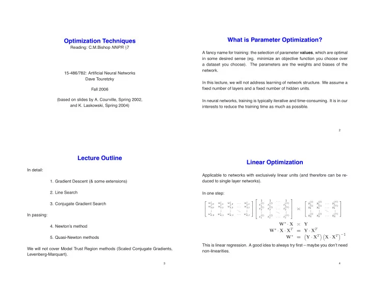
Applicable to networks with exclusively linear units (and therefore can be re- duced to single layer networks). In one step:

  

w∗

1,0

w∗

1,1

w∗

1,2

. . . w∗

1,I

w∗

2,0

w∗

2,1

w∗

2,2

. . . w∗

2,I

. . . . . . . . . ... . . . w∗

K,0

w∗

K,1

w∗

K,2

. . . w∗

K,I

       

1 1 . . . 1 x(1)

1

x(2)

1

. . . x(N)

1

x(1)

2

x(2)

2

. . . x(N)

2

. . . . . . ... . . . x(1)

I

x(2)

I

. . . x(N)

I

    

≍

  

y(1)

1

y(2)

1

. . . y(N)

1

y(1)

2

y(2)

2

. . . y(N)

2

. . . . . . ... . . . y(1)

K

y(2)

K

. . . y(N)

K

  

W∗ · X ≍ Y W∗ · X · XT = Y · XT W∗ =

• Y · XT

X · XT −1 This is linear regression. A good idea to always try first – maybe you don’t need non-linearities.

4

SLIDE 2

Try It In Matlab

>> W = [1 2 3]; >> x = [ ones(1,50); rand(2,50)]; >> y = W*x; >> W_star = (y*x’) * inv(x*x’) W_star = 1.0000 2.0000 3.0000 >> W_hat = y * pinv(x) W_hat = 1.0000 2.0000 3.0000

5

Non-linear Optimization

Given a fixed neural network architecture with non-linearities, we seek iterative algorithms which implement a search in parameter space: w(τ+1) = w(τ) + ∆w(τ) w ∈ ℜW At each timestep τ, ∆w(τ) is chosen to reduce an objective (error) function E({x, t}; w). For example, for a network with K linear output units, the appro- priate choice is the sum-of-squares error: E = 1 2

N

• n=1

K

• k=1

yk(xn; w) − tn k 2

where N is the number of patterns.

6

The Parameter Space

• y1

· · ·

• yk

· · ·

• yK

1

• z1
• z2
• z3
• z4
• · · ·
• zj
• · · ·
• zJ
• 1
• x1
• x2
• · · ·
• xi
• · · ·
• xI
• W2

=

 

w(2)

0,1

w(2)

1,1

· · · w(2)

J,1

. . . . . . ... . . . w(2)

0,K

w(2)

1,K

· · · w(2)

J,K

 

∈ ℜ(K,J+1) W1 =

 

w(1)

0,1

w(1)

1,1

· · · w(1)

I,1

. . . . . . ... . . . w(1)

0,J

w(1)

1,J

· · · w(1)

I,J

 

∈ ℜ(J,I+1) Want to think of (and operate on) weight matrices as a single vector: w = mapping (W1, W2) ∈ ℜW, W = J (I + 1) + K (J + 1) Doesn’t matter what mapping is, as long as we can reverse it when necessary.

7

Approximating Error Surface Behaviour

Holding the dataset {x, t} fixed, consider a second order Taylor series expan- sion of E(w) about a point w0: E(w) = E(w0) + (w − w0)Tb + 1 2(w − w0)TH(w − w0) (1) where b is the gradient of E|w0 and H is the Hessian of E|w0: b ≡ ∇E|w0 =

 

∂E ∂w1

. . .

∂E ∂wW

  w0

H ≡ ∇2E|w0 =

 

∂2E ∂w2

1

· · ·

∂2E ∂w1∂wW

. . . ... . . .

∂2E ∂wW ∂w1

· · ·

∂2E ∂w2

W

  w0

In a similar way, we can define a first order approximation to the gradient: ∇E|w = b + H (w − w0) (2)

8

SLIDE 3

Near a Minimum

How does the error surface behave near a minimum w∗? The gradient b ≡ ∇E|w0 → 0, so the shape of the error surface is uniquely determined (to second order) by the Hessian: E(w) = E(w∗) + 1 2(w − w∗)TH(w − w∗) H =

• 1

1

• H =
• 1

2

• H =
• 2

1 1 3

• 9

General Algorithm Structure

STEP 1. τ = 0. Initialize w(0). Covered in §7.4. while (TRUE) { STEP 2. Compute ∆w(τ). Update w(τ+1) = w(τ) + ∆w(τ). Update τ = τ + 1. STEP 3. If termination reached (covered in next lecture), exit and return w∗ = w(τ). }

10

Gradient Descent Search

∆w(τ) = η · −∇E|w(τ)

• (search) direction

(3) As we’ve seen, the step size η is not a function of w(τ) and is known in as the learning rate. In the most basic form of Gradient Descent Search, it’s just a constant, and you have to set it by hand. At each timestep τ, ∆w is a function of the current true gradient only. The search history is ignored. As we will see, later algorithms will exploit the search history.

11

Conditions for Convergence

Under what conditions will we converge to a minimum? Hard to say. But if we assume a quadratic error surface, we can answer this if we rotate into the eigenspace of H and move such that w∗ → 0 (assume we are doing a post-mortem and know both H and w∗).

w w∗ w

12

SLIDE 4

The Eigenspace of H

Since H = HT, its eigenvectors Hui = λiui i ∈ [1, W] (4) form a complete orthonormal basis of ℜW. Why? Because for any pair, uj and uk, j = k, uT

j Huk

= λkuT

j uk

• uT

k Huj T

=

• λjuT

k uj T

⇒ =

• λk − λj
• uT

k uj

So for λk = λj, the eigenvectors are orthogonal. Otherwise, they define a plane in which all vectors are eigenvectors corresponding to λk = λj, so we can choose any two orthogonal vectors which span this plane. Then normalize all ui to have unit length.

13

The Gradient in the Eigenspace of H

We’ve successfully constructed a new (more useful) orthonormal basis of our

• riginal space. We can express any original vector w in these new coordinates

as: w = w∗ +

W

• i=1

αiui ⇔ w − w∗ =

W

• i=1

αiui (5) Recalling Eq 2, we compute the gradient of our second order approximation at w using Eq 5 and simplify with Eq 4: ∇E|w = H

w − w∗

= H

W

• i=1

αiui =

W

• i=1

αiλiui (6)

14

Weight Update in the Eigenspace of H

Let’s transform our weight increment from the original coordinate system to the new coordinates using Eq 5: ∆w(τ) = w(τ+1) − w(τ) =

 w∗ + W

• i=1

α(τ+1)

i

ui

  −  w∗ + W

• i=1

α(τ)

i

ui

 

=

W

• i=1

∆α(τ)

i

ui Recall that for Gradient Descent Search, ∆w(τ) = −η∇E|w(τ) = −η∇E|w(τ) (7) = −η

W

• i=1

α(τ)

i

λiui (8) where the equality in line 7 holds because we have been assuming a quadratic error surface, and Eq 8 follows from Eq 6.

15

Gradient Descent Search Convergence, cont’d...

By inspection from Eqs 7 & 8, ∆αi = −ηλiαi. So, in the new coordinate system, α(τ+1)

i

= α(τ)

i

+ ∆α(τ)

i

= (1 − ηλi) α(τ)

i

(9) Remember that we want to converge to 0 (w∗ in the original basis). After R timesteps, lim

R→∞ α(R) i

= lim

R→∞ (1 − ηλi)R α(0) i

(10) = (11) ⇒ lim

R→∞ w(R)

= w∗ (12) iff |1 − ηλi| < 1 (13) Finally (it took 5 slides). We will converge to the minimum if and only if η <

2 λmax.

16

SLIDE 5

Speed of Convergence

Governed by how long it takes each of the (1 − ηλi)R to decay to 0, under the constraint that η < 2/λmax. The larger λi, the closer (1−ηλi) is to 0 and so the faster will (1−ηλi)R decay. Therefore convergence is slowest for the smallest λi. Specifically, convergence will be governed by how close the following gets to zero: max

λi

(1 − ηλi) = max

λi

• 1 −

2 λmax λi

• =

1 − 2λmin λmax So the closer λmin and λmax are, the faster we will find the minimum. The situation becomes even less optimistic when we drop our assumption of a quadratic error surface. Then H may not only be ill-conditioned, it is generally different for every point in weight space.

17

Gradient Descent Search Pros & Cons

Straightforward, iterative, tractable, locally optimal descent in error — see demo. But we have four main objections:

• 1. Cannot avoid local minima, and cannot escape them (but may occasionally
• vershoot them).
• 2. Cannot guarantee a scalable bound on time complexity. Rather, speed to

convergence governed by the condition number of the local Hessian, which may be changing from point to point.

• 3. Step size constant, not sensitive to local topology. Furthermore, has to be

carefully set by hand.

• 4. Search direction only locally optimal.

18

Addressing the Limitations

The rest of this lecture. Want to find techniques for adapting the step size and for making direction decisions which are optimal in more than just a local sense.

w/ both algorithms algorithms w/ algorithms w/

non-local direction selection Gradient Descent adaptive step size

Also want to try to limit time complexity, storage complexity, and the number of parameters which must be externally set by hand. Sadly, can’t do much about local minima.

19

Avoiding/Escaping Local Minima

The only way to avoid getting trapped in a local minimum is to accidentally step

• ver it (with a step size or inertia which is locally too high). The likelihood of

this occurring depends on the optimization technique. Leaving local minima is possible by random perturbation. Simulated Annealing and Genetic Algorithms are examples, but we won’t cover them in this lecture. Stochastic Gradient Descent is a form of injecting randomness into Gradient Descent.

20

SLIDE 6

Stochastic Gradient Descent

Rather than computing the error gradient for all patterns, could go through the patterns sequentially, one pattern per iteration. ∆w(τ) = ηs · −∇En|w(τ) In contrast to the batch version, this offers the possibility of escaping from local minima. Likely to be more efficient for datasets with high redundancy. Note that value of ηs may be different than for the η in the batch version. Strictly speaking, it’s stochastic only if you choose the patterns randomly.

21

Using Learning Rate Schedules

In practice, error vs epoch curves exhibit distinct regions where some definite statements about the suitability of the learning rate can be made.

E epoch

Once you are familiar with how your neural network is training you will be able to guess at several learning rates, which you will want to kick in at specific times. You’ll see this in an upcoming homework assignment.

22

Adding Momentum

∆w(τ) = −η∇E|w(τ) + µ∆w(τ−1) (14) µ = 0.0 µ = 0.1 µ = 0.2 Generally leads to significant improvements in speed of convergence. See demo. Escape from local minima possible. Yet another parameter to set manually.

23

Line Search

Let’s try to do something about the step size. At every timestep τ, run a small subalgorithm:

• 1. Choose a search direction as in gradient descent:

d(τ) = −∇E|w(τ)

• 2. Minimize the error along the search direction:

λ(τ) = argminλ>0 E(w(τ) + λd(τ)) NOTE: This is a one-dimensional problem!

• 3. Return the weight update:

∆w(τ) = λ(τ) · d(τ)

24

SLIDE 7

Minimizing Error in 1 Dimension

λ1 = 0, E(λ1) λ3, E(λ3) λ2, E(λ2) λ∗, E(λ∗) λ E(λ)

• 2a. Pick 3 values λ1 = 0 < λ2 < λ3 such that E(λ2) is smallest. Enter inner loop:
• 2b. Fit points to a parabola Ei = aλ2

i + bλi + c, 1≤i≤3 (linear regression).

• 2c. Compute λ∗ = − b

2a, the parabola’s minimum; evaluate E(λ∗).

• 2d. If E(λ∗) ≈ E(λ2), return λ∗ and exit.
• 2e. Else replace {λ2, E(λ2)} by {λ∗, E(λ∗)} and goto 2b.

25

A Bird’s Eye View of Line Search

TOP VIEW CONTOURS TOP VIEW NEGATIVE GRADIENT SIDE VIEW ELEVATION

As we move in a straight line, the gradient beneath our feet keeps changing (we’re on a curved surface). Line search will stop us when the component of the gradient parallel to our direction of travel is zero. Consequence: successive directions in Line Search are perpendicular.

26

How good are ⊥ Search Directions?

Gradient Descent, large η Gradient Descent, small η Line Search

In Gradient Descent Search, we may be oscillating back and forth such that the angle between successive directions is almost 180 degrees. But we have the

• pportunity, by keeping η small, to follow the optimal path to the minimum.

27

Orthogonal Search Directions, cont’d...

In Line Search, by contrast, we are stuck with successive directions that are at exactly 90 degrees to each other, always (see demo). This is an immutable fact, regardless of the topology. This means that, even for a 2-dimensional quadratic error surface, we will take many steps to converge. The picture is far messier when we consider a W-dimensional parameter space with W large (ALVINN W ≈ 4000). Throw away the quadratic assumption, and things get messier still.

28

SLIDE 8

Line Search Pros & Cons

• 1. No parameters to set by hand, yay!
• 2. Successive search directions are orthogonal. Don’t quite know whether this

is a blessing or a curse. Seems better than Gradient Descent Search, but still somehow unsatisfactory. Could take a long time to converge.

• 3. Line search requires that we evaluate E(λ) many times per iteration. Each

time we have to do a full forward propagation of the training set through our neural network.

29

What Can We Do About the ⊥ Directions

d(1) d(3) d(2)

Note that, at each step, we choose a direction which ends up undoing the progress we made on the previous step. We’ll have to make it up again later.

30

Conjugate Gradient Search

d(1) d(3) d(2) d(4) d(2)∗

At τ = 2, we would really like to take direction d(2)∗ instead. This would avoid us having to repeat progress already made during step 1 on the next step.

31

Conjugate Gradients, Theory Part 1

At w(τ+1),

• −∇E|w(τ+1)

T d(τ) = 0

(15) Once we choose the next direction d(τ+1) and begin a line search step, our position along that direction will be w(τ+1) +λd(τ+1) and our gradient at that position will be ∇E|w(τ+1)+λd(τ+1). To a first order approximation, ∇E|w(τ+1)+λd(τ+1) = ∇E|w(τ+1) +

• w(τ+1) + λd(τ+1) − w(τ+1)T · H

= ∇E|w(τ+1) + λd(τ+1) TH (16)

32

SLIDE 9

Conjugate Gradients, Theory Part 2

We want to have chosen our next direction d(τ+1) such that, to a first order approximation, our gradient along this direction will remain orthogonal to the previous direction d(τ):

• −∇E|w(τ+1)+λd(τ+1)

T d(τ)

= (17) We can substitute Eq 16 into Eq 17 −

• ∇E|w(τ+1) + λd(τ+1) TH

T d(τ)

=

• −∇E|w(τ+1)

T d(τ) − λd(τ+1) THd(τ)

= d(τ+1) THd(τ) = (18) where the first term on the second line cancels due to Eq 15. Pairs of directions d(τ+1) and d(τ) for which Eq 18 holds are called mutually

• conjugate. They are orthogonal in the (rotated) space where H is the identity.

33

Constructing the Next Conjugate Direction

Note that the new direction is a linear combination of the current negative gra- dient and the previous search direction: d(τ+1) = −∇E|w(τ+1) + β(τ)d(τ) (19) We can solve for β(τ) by first taking the transpose of Eq 19 and then multiplying by Hd(τ) and imposing Eq 18: d(τ+1) THd(τ) = −

• ∇E|w(τ+1)

T Hd(τ) + β(τ)d(τ) THd(τ)

This yields β(τ) =

• ∇E|w(τ+1)

T Hd(τ)

d(τ) T Hd(τ) (20)

34

Can Computation of H Be Avoided?

H is costly to compute, and so we would like to avoid its evaluation at every

• step. Under a quadratic error surface assumption, it can be shown that Eq 20

reduces to the Polak-Ribiere formula: β(τ) =

• ∇E|w(τ+1)

T

∇E|w(τ+1) − ∇E|w(τ)

• ∇E|w(τ)

T ∇E|w(τ)

(21) There are several competing expressions; this one is believed to generalize better to non-quadratic error surfaces.

35

The Conjugate Gradient Search Algorithm

Just like the inner-loop subalgorithm for Line Search. Prior to incrementing τ:

• 1a. Compute −∇E|w(τ+1) (one back propagation).
• 1b. For τ = 1, set β(1) = 0. Else evaluate β(τ) using Eq 21.
• 1c. Evaluate d(τ+1) using Eq 19.
• 1d. Update τ = τ + 1.

Check out the demo.

36

SLIDE 10

How Does Conjugate Gradient Search Stack Up?

If we had a quadratic error surface, we would need to perform at most W weight updates before reaching the minimum. 2-D toy problems will be solved two steps. Need to store previous search direction (O(W) storage). But this isn’t so bad. Require multiple evaluations of the error (forward propagations through the neural network) during line error minimization. We need an accurate line error minimization routine since we are using our position to set up a conjugate system. In Line Search this wasn’t so important. Still no chance of leaving poor local minima.

37

Newton’s Method

For a quadratic error surface, our 1st order approximation to the gradient (Eq 2) is the true gradient. Expanding about w∗ and noting that the gradient at w∗ is 0: ∇E|w = H

w − w∗

(22) Eq 22 can be solved directly w∗ = w − H−1∇E|w and the corresponding weight update, ∆w = −H−1∇E|w is called the Newton step.

38

Newton’s Method: Caveats

• 1. The error surface isn’t really quadratic; algorithm must be applied iteratively

like everything else.

• 2. Computation of H−1 is O(W 3).
• 3. Points 1 and 2 together should make you cringe. In ALVINN, with 4000

parameters, that’s 6.4 × 1010 computations per iteration. 4. Additionally, if H isn’t positive definite, the algorithm could fail to find a minimum.

39

Quasi-Newton Methods

AIM: Since exact computation of H−1 is so expensive, let’s find an approxi- mation G(τ) which is cheaper to compute and simultaneously ensure that it is positive definite. At τ = 1, initialize G(1) = I. At each timestep τ, generate a new G(τ). The G(τ) are a sequence of in- creasingly better approximations to H−1. Then apply the Newton step weight update. Use line minimization just to make sure we’re not taken outside of the range of validity of our quadratic approxi- mation: ∆w(τ) = −λ(τ)G(τ)∇E|w(τ)

40

SLIDE 11

Computing G(τ+1) using BFGS

The Broyden-Fletcher-Goldfarb-Shanno procedure is the most well-known quasi- Newton method of H−1 approximation: p = w(τ+1) − w(τ) v = ∇E|w(τ+1) − ∇E|w(τ) u = p pTv − G(τ)v vTG(τ)v G(τ+1) = G(τ) + ppT pTv −

• G(τ)v
• vTG(τ)

vTG(τ)v +

• vTG(τ)v
• uuT

41

Technique Performance Comparison

Taken from www.mathworks.com Neural Networks Toolbox User Guide. gdx = Variable Rate Gradient Descent, cgb = Conjugate Gradient Search with restarts, scg = Scaled Conjugate Gradient Search, rp = Resilient Backprop, lm = Levenberg-Marquart

42

What We’ve Covered

algorithms w/ algorithms w/

Gradient Descent step size adaptive Line Search Gradient Descent with Variable Learning Rate selection direction non-local Gradient Descent with Momentum Gradient Conjugate

43