what i am after
play

what I am after Statistical modelling and analysis do not from - PDF document

Why graphical models in R? what I am after Statistical modelling and analysis do not from gR2002 respect boundaries of model classes Software should encourage and support good practice - and graphical models are good practice!


  1. Why graphical models in R? ‘what I am after’ • Statistical modelling and analysis do not from gR2002 respect boundaries of model classes • Software should encourage and support good practice - and graphical models are good practice! • Data analysis - model-based • R for ‘reference implementation’ of new Peter Green, methodology University of Bristol, UK • Open software Contingency Markov Spatial Questions tables chains statistics • Scope? – Digram, MIM, CoCo, TETRAD, Hugin, Genetics BUGS? – Determined by classes of model, or Regression Graphical models classes of algorithm? • Market? AI – Statistics researcher, statistics MSc, arbitrary Excel user? • Delivery? Statistical Sufficiency Covariance – R package(s), with C code? physics selection 
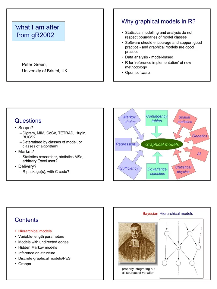
Bayesian Hierarchical models Contents • Hierarchical models • Variable-length parameters • Models with undirected edges • Hidden Markov models • Inference on structure • Discrete graphical models/PES • Grappa properly integrating out all sources of variation

  2. Repeated measures on children's Repeated measures on children's weights weights, continued ( α i β , ) • Children i=1,2,…,k have their weights • Suppose that vary across the i measured on n i occasions, t ij ,j=1,2,…n i population according to obtaining weights y ij . 2 2 α ~ N ( µ , σ ) β ~ N ( µ , σ ) i α α i β β • Suppose that, for each child, we have a linear growth equation, with • A Bayesian completes the model by independent normal errors 2 2 2 ( µ , σ , µ , σ , σ ) specifying priors on α α β β + 2 y ~ N ( α β t , σ ) ij i i ij Measurement error Graph for children’s weights Explanatory variables µ σ µ σ α α β β X subject to error - we σ { ij t } α β { } { } only observe i i U on most cases { y } ij Contents Mixture modelling k DAG for a • Hierarchical models mixture model • Variable-length parameters w • Models with undirected edges k θ ∑ θ y ~ w f ( y | ) • Hidden Markov models j j j = 1 • Inference on structure • Discrete graphical models/PES • Grappa y

  3. Measurement error using mixture Mixture modelling model for population k DAG for a length= k mixture model w k θ ∑ θ y ~ w f ( y | ) z j j = j 1 = θ ( y | z j ) ~ f ( y | ) y j = ) = p ( z j w j value set ={1,2,…, k } Modelling with undirected Contents graphs • Hierarchical models Directed acyclic graphs are a natural representation of the way we usually • Variable-length parameters specify a statistical model - directionally: • Models with undirected edges • Hidden Markov models • disease → symptom • Inference on structure • past → future • Discrete graphical models/PES • parameters → data ….. • Grappa However, sometimes (e.g. spatial models) there is no natural direction Scottish lip cancer data Scottish lip cancer data (2) The data include The rates of lip cancer in 56 counties in • the observed and expected cases (expected Scotland have been analysed by numbers based on the population and its age Clayton and Kaldor (1987) and Breslow and sex distribution in the county), and Clayton (1993) • a covariate measuring the percentage of the population engaged in agriculture, fishing, or forestry, and (the analysis here is based on the example in the • the "position'' of each county expressed as WinBugs manual) a list of adjacent counties.

  4. Scottish lip cancer data (3) Model for lip cancer data (1) Graph regression coefficient County Obs Exp x SMR Adjacent cases cases (% in counties covariate agric.) random spatial effects 1 9 1.4 16 652.2 5,9,11,19 2 39 8.7 16 450.3 7,10 expected counts ... ... ... ... ... ... 56 0 1.8 10 0.0 18,24,30,33,45,55 observed counts Model for lip cancer data Bugs code for lip cancer data (2) Distributions µ O ~ Poisson ( ) • Data: model i i { • Link function: b[1:regions] ~ car.normal(adj[], weights[], num[], tau) µ = + α + α + b.mean <- mean(b[]) log log E x / 10 b i i 0 1 i i for (i in 1 : regions) { O[i] ~ dpois(mu[i]) • Random spatial effects: log(mu[i]) <- log(E[i]) + alpha0 + alpha1 * x[i] / 10 + b[i] ∑ τ ∝ τ n / 2 − τ − 2 SMRhat[i] <- 100 * mu[i] / E[i] p ( b ,..., b | ) exp( ( b b ) / 4 ) 1 n i j } Note: declarative, i ~ j alpha1 ~ dnorm(0.0, 1.0E-5) rather than alpha0 ~ dflat() • Priors: tau ~ dgamma(r, d) procedural α 0 α τ Γ , ~ Uniform ~ ( r , d ) sigma <- 1 / sqrt(tau) language 1 } Bugs code for lip cancer data Bugs code for lip cancer data model model { { b[1:regions] ~ car.normal(adj[], weights[], num[], tau) b[1:regions] ~ car.normal(adj[], weights[], num[], tau) b.mean <- mean(b[]) b.mean <- mean(b[]) µ O ~ Poisson ( ) for (i in 1 : regions) { for (i in 1 : regions) { µ = + α + α + log log E x / 10 b i i O[i] ~ dpois(mu[i]) O[i] ~ dpois(mu[i]) i i 0 1 i i log(mu[i]) <- log(E[i]) + alpha0 + alpha1 * x[i] / 10 + b[i] log(mu[i]) <- log(E[i]) + alpha0 + alpha1 * x[i] / 10 + b[i] SMRhat[i] <- 100 * mu[i] / E[i] SMRhat[i] <- 100 * mu[i] / E[i] } } alpha1 ~ dnorm(0.0, 1.0E-5) alpha1 ~ dnorm(0.0, 1.0E-5) alpha0 ~ dflat() alpha0 ~ dflat() tau ~ dgamma(r, d) tau ~ dgamma(r, d) sigma <- 1 / sqrt(tau) sigma <- 1 / sqrt(tau) } }

  5. Bugs code for lip cancer data Bugs code for lip cancer data ∑ p ( b ,..., b | τ ) ∝ τ n / 2 exp( − τ ( b − b ) 2 / 4 ) model model 1 n i j { i ~ j { b[1:regions] ~ car.normal(adj[], weights[], num[], tau) b[1:regions] ~ car.normal(adj[], weights[], num[], tau) b.mean <- mean(b[]) b.mean <- mean(b[]) for (i in 1 : regions) { for (i in 1 : regions) { O[i] ~ dpois(mu[i]) O[i] ~ dpois(mu[i]) log(mu[i]) <- log(E[i]) + alpha0 + alpha1 * x[i] / 10 + b[i] log(mu[i]) <- log(E[i]) + alpha0 + alpha1 * x[i] / 10 + b[i] SMRhat[i] <- 100 * mu[i] / E[i] SMRhat[i] <- 100 * mu[i] / E[i] } } alpha1 ~ dnorm(0.0, 1.0E-5) alpha1 ~ dnorm(0.0, 1.0E-5) alpha0 ~ dflat() alpha0 ~ dflat() τ Γ ~ ( r , d ) tau ~ dgamma(r, d) tau ~ dgamma(r, d) sigma <- 1 / sqrt(tau) sigma <- 1 / sqrt(tau) } } WinBugs for lip cancer data WinBugs for lip cancer data alpha1 sample: 7000 Dynamic traces for some parameters: 4.0 Posterior densities 3.0 alpha1 for some parameters: 2.0 0.75 0.5 1.0 0.25 0.0 0.0 -0.25 -0.5 0.0 0.5 1.0 16600 16650 16700 16750 16800 16850 16900 16950 iteration mu[1] sample: 7000 tau sample: 7000 tau mu[1] 0.3 0.8 6.0 15.0 0.6 4.0 10.0 0.2 0.4 5.0 2.0 0.1 0.2 0.0 0.0 0.0 16600 16650 16700 16750 16800 16850 16900 16950 0.0 16600 16650 16700 16750 16800 16850 16900 16950 iteration iteration 0.0 5.0 10.0 15.0 0.0 2.0 4.0 Contents Hidden Markov models e.g. Hidden Markov chain • Hierarchical models (DLM, state space model) • Variable-length parameters • Models with undirected edges z 0 z 1 z 2 z 3 z 4 hidden • Hidden Markov models • Inference on structure • Discrete graphical models/PES y 1 y 2 y 3 y 4 observed • Grappa

Download Presentation
Download Policy: The content available on the website is offered to you 'AS IS' for your personal information and use only. It cannot be commercialized, licensed, or distributed on other websites without prior consent from the author. To download a presentation, simply click this link. If you encounter any difficulties during the download process, it's possible that the publisher has removed the file from their server.

Recommend


More recommend