
SLIDE 1
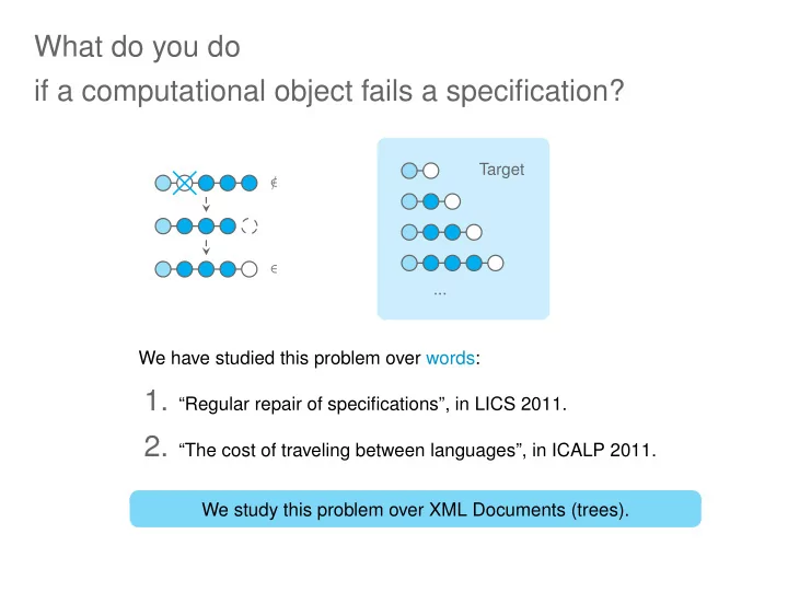
What do you do if a computational object fails a specification?
∉ ∈ ... Target
We have studied this problem over words:
- 1. “Regular repair of specifications”, in LICS 2011.
- 2. “The cost of traveling between languages”, in ICALP 2011.
We study this problem over XML Documents (trees).