Weighted reduced order methods for parametrized PDEs with random - PowerPoint PPT Presentation
Weighted reduced order methods for parametrized PDEs with random inputs Francesco Ballarin 1 , Davide Torlo 2 , Luca Venturi 3 , Gianluigi Rozza 1 1 mathLab, Mathematics Area, SISSA, Trieste, Italy 2 Universitt Zrich, Switzerland 3 Courant
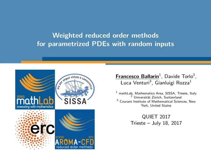
Weighted reduced order methods for parametrized PDEs with random inputs Francesco Ballarin 1 , Davide Torlo 2 , Luca Venturi 3 , Gianluigi Rozza 1 1 mathLab, Mathematics Area, SISSA, Trieste, Italy 2 Universität Zürich, Switzerland 3 Courant Institute of Mathematical Sciences, New York, United States QUIET 2017 Trieste – July 18, 2017
Introduction and outline of the talk • Parametrized partial differential equations (elliptic, mainly); • parameters → random inputs ; • evaluation of some statistics on the solution u , e.g. E [ u ]; • using reduced order models to accelerate Monte Carlo methods: • how to weight solutions during the construction of the ROM; • how to sample the parameter space during the construction of the ROM; • weighted reduced basis method [P. Chen et al., SIAM J. Numer. Anal., 2013], [ D. Torlo et al., 2017] • weighted proper orthogonal decomposition method [ L. Venturi et al., 2017] • combination with reduced order stabilization techniques for advection dominated problems. F. Ballarin, D.Torlo, L. Venturi, G. Rozza Weighted ROMs for parametrized PDEs with random inputs 1/ 27
Parametrized stochastic partial differential equations • Ω ⊂ R d , d = 1 , 2 , 3, a domain ; • ( A , F , P ) a complete probability space; • µ : ( A , F ) → ( D , B ), a random vector : • D ⊂ R p , a compact set in the parameter space ; • µ ( ω ) = ( µ 1 ( ω ) , . . . , µ p ( ω )) independent identically distributed and absolutely continuous random variables ; • H 1 0 (Ω) ⊂ V ⊂ H 1 (Ω); • S (Ω) := L 2 ( A ) � V ; • u : Ω × A → R , i.e. u ∈ S (Ω), a random field ; • elliptic PDE, e.g., advection–diffusion stochastic equation − ε ( µ ( ω ))∆ u ( µ ( ω )) + β ( µ ( ω )) · ∇ u ( µ ( ω )) = f ( µ ( ω )) in Ω , s.t. suitable boundary conditions on ∂ Ω. F. Ballarin, D.Torlo, L. Venturi, G. Rozza Weighted ROMs for parametrized PDEs with random inputs 2/ 27
Reduced basis methods: the greedy algorithm Sample Ξ train ⊂ D Pick arbitrary µ 1 ∈ Ξ train Define S 0 = ∅ , X RB = ∅ 0 for N = 1 , . . . , N max Perform a PDE solve to compute u ( µ N ) S N = S N − 1 ∪ { µ N } X RB = X RB N − 1 ⊕ { u ( µ N ) } N [ ε N , µ N ] = max µ ∈ Ξ train ∆ N ( µ ) if ε N ≤ tol break end end where ∆ N ( µ ) is a sharp, inexpensive a posteriori error bound for � u ( µ ) − u N ( µ ) � V , being u N ( µ ) the RB solution of dimension N . J. S. Hesthaven, G. Rozza, B. Stamm. Certified Reduced Basis Methods for Parametrized Partial Differential Equations . SpringerBriefs in Mathematics. Springer International Publishing, 2015 F. Ballarin, D.Torlo, L. Venturi, G. Rozza Weighted ROMs for parametrized PDEs with random inputs 3/ 27
Weighted reduced basis methods: motivation The introduction of a weight in the greedy algorithm reflects our desire of minimizing the squared norm error of the reduced order approximation, i.e. � E � � � u − u N � 2 � u ( µ ( ω )) − u N ( µ ( ω )) � 2 = V dP ( ω ) = V A � � u ( µ ) − u N ( µ ) � 2 = V ρ ( µ ) d µ , D being ρ : A → R the probability density distribution of µ . Thus, � E � � � u − u N � 2 ∆ N ( µ ) 2 ρ ( µ ) d µ , ≤ V D This motivates the choice of the weight � w ( µ ) = ρ ( µ ) and the introduction of the error bound � ∆ w N ( µ ) := ∆ N ( µ ) ρ ( µ ) . P. Chen, A. Quarteroni, and G. Rozza. A weighted reduced basis method for elliptic partial differential equations with random input data. SIAM Journal on Numerical Analysis, 51(6):3163–3185, 2013. F. Ballarin, D.Torlo, L. Venturi, G. Rozza Weighted ROMs for parametrized PDEs with random inputs 4/ 27
Weighted reduced basis methods: the greedy algorithm Properly sample Ξ train ⊂ D Pick arbitrary µ 1 ∈ Ξ train Define S 0 = ∅ , X RB = ∅ 0 for N = 1 , . . . , N max Perform a PDE solve to compute u ( µ N ) S N = S N − 1 ∪ { µ N } X RB = X RB N − 1 ⊕ { u ( µ N ) } N [ ε N , µ N ] = max µ ∈ Ξ train ∆ w N ( µ ) if ε N ≤ tol break end end P. Chen, A. Quarteroni, and G. Rozza. A weighted reduced basis method for elliptic partial differential equations with random input data. SIAM Journal on Numerical Analysis, 51(6):3163–3185, 2013. F. Ballarin, D.Torlo, L. Venturi, G. Rozza Weighted ROMs for parametrized PDEs with random inputs 5/ 27
Reduction by proper orthogonal decomposition Sample Ξ train ⊂ D for N = 1 , . . . , M ≡ card(Ξ train ) Pick the N -th element µ N in Ξ train Perform a PDE solve to compute u ( µ N ) end Assemble the correlation matrix C ∈ R M × M , with entries C ij = 1 M ( u ( µ i ) , u ( µ j )) V , i , j = 1 , . . . , M Compute the eigenvalues of C , sort them in decreasing order, and retain the ones that are larger than tol , as well as their corresponding eigenfunctions. J. S. Hesthaven, G. Rozza, B. Stamm. Certified Reduced Basis Methods for Parametrized Partial Differential Equations . SpringerBriefs in Mathematics. Springer International Publishing, 2015 F. Ballarin, D.Torlo, L. Venturi, G. Rozza Weighted ROMs for parametrized PDEs with random inputs 6/ 27
Weighted proper orthogonal decomposition: motivation Standard POD algorithm results in the optimal N -dimensional subspace of V which minimizes � M � � 1 � u ( µ i ) − u N ( µ i ) � 2 M V i =1 Now, consider a weight w : D → R + and minimize instead � M � � 1 � 2 � u ( µ i ) − u N ( µ i ) w ( µ i ) M V i =1 In practice, this amounts to computing the eigenvalues of the following weighted correlation matrix 1 2 C C w = W where W = diag { w ( µ 1 ) , . . . , w ( µ M ) } . L. Venturi, F. Ballarin, and G. Rozza. Weighted POD–Galerkin methods for parametrized partial differential equations in uncertainty quantification problems. In preparation, 2017 F. Ballarin, D.Torlo, L. Venturi, G. Rozza Weighted ROMs for parametrized PDEs with random inputs 7/ 27
Weighted proper orthogonal decomposition: offline stage Sample Ξ train ⊂ D for N = 1 , . . . , M ≡ card(Ξ train ) Pick the N -th element µ N in Ξ train Perform a PDE solve to compute u ( µ N ) end Assemble the weighted correlation matrix C w ∈ R M × M . Compute the eigenvalues of C w , sort them in decreasing order, and retain the ones that are larger than tol , as well as their corresponding eigenfunctions. L. Venturi, F. Ballarin, and G. Rozza. Weighted POD–Galerkin methods for parametrized partial differential equations in uncertainty quantification problems. In preparation, 2017 F. Ballarin, D.Torlo, L. Venturi, G. Rozza Weighted ROMs for parametrized PDEs with random inputs 8/ 27
Weighted proper orthogonal decomposition: choice of the weight • the choice w ( µ ) ≡ ρ ( µ ) with µ i ∼ Unif( D ) results in the minimization of � M � � 1 � 2 � u ( µ i ) − u N ( µ i ) ρ ( µ i ) V ≈ M i =1 � V ρ ( µ ) d µ = E � � � u ( µ ) − u N ( µ ) � 2 � u − u N � 2 ≈ , V D i.e. a Uniform Monte Carlo quadrature for the squared norm error of the reduced order approximation. • the choice w ( µ ) ≡ 1 with µ i ∼ Distribution( D ) results in the minimization of � M � � 1 � 2 � u ( µ i ) − u N ( µ i ) V ≈ M i =1 � V dP ( ω ) = E � � � u ( µ ( ω )) − u N ( µ ( ω )) � 2 � u − u N � 2 ≈ , V D i.e. a Monte Carlo quadrature for the squared norm error of the reduced order approximation. L. Venturi, F. Ballarin, and G. Rozza. Weighted POD–Galerkin methods for parametrized partial differential equations in uncertainty quantification problems. In preparation, 2017 F. Ballarin, D.Torlo, L. Venturi, G. Rozza Weighted ROMs for parametrized PDEs with random inputs 9/ 27
Weighted proper orthogonal decomposition: choice of weight and sampling • the previous choices resulted in the minimization of a (Uniform) Monte Carlo quadrature for the squared norm error of the reduced order approximation. • moreover, we can consider more general quadrature rules of the form � M ω i f ( x i ) U ( f ) = i =1 for every integrable function f : D → R , where x 1 , . . . , x M ∈ D are the nodes of the quadrature and ω 1 , . . . , ω M are the respective weights. This results in the following approximation: � M E � � � � ≈ 1 � u ( x i ) − u N ( x i ) � 2 � u − u N � 2 ω i ρ ( x i ) V V M i =1 which motivates the following choice: • sample the parameter spaces with { µ i ≡ x i } M i =1 , and • weigh as w ( µ i ) ≡ ω i ρ ( µ i ), i = 1 , . . . , M . L. Venturi, F. Ballarin, and G. Rozza. Weighted POD–Galerkin methods for parametrized partial differential equations in uncertainty quantification problems. In preparation, 2017 F. Ballarin, D.Torlo, L. Venturi, G. Rozza Weighted ROMs for parametrized PDEs with random inputs 10/ 27
Test case 1: 3 × 3 thermal block w i RB | Ξ train | Standard 1 2000 � Weighted - Unif. ρ i 2000 � Weighted - Distr. ρ i 2000 w i POD | Ξ train | Standard 1 500 Monte-Carlo 1 500 ρ i Uniform M.-C. 2000 ω i Gauss-Jacobi 512 ω i ρ i Gauss-Legendre 512 � � � 9 µ i ∇ u ( µ ) · ∇ v dx = v dx , ∀ v ∈ V Ω i Ω i =1 α = β = 10 α = β = 75 µ ∈ [1 , 3] 9 : µ i − 1 ∼ Beta( α, β ) 2 F. Ballarin, D.Torlo, L. Venturi, G. Rozza Weighted ROMs for parametrized PDEs with random inputs 11/ 27
Recommend
More recommend
Explore More Topics
Stay informed with curated content and fresh updates.
