
SLIDE 1
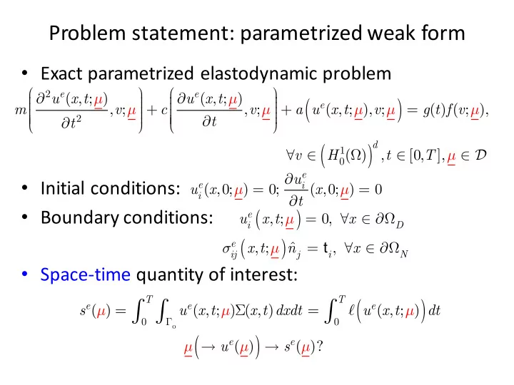
Problem statement: parametrized weak form
- Exact parametrized elastodynamic problem
- Initial conditions:
- Boundary conditions:
- Space-time quantity of interest:
m ∂2ue(x,t;µ) ∂t2 ,v;µ ⎛ ⎝ ⎜ ⎜ ⎜ ⎜ ⎜ ⎞ ⎠ ⎟ ⎟ ⎟ ⎟ ⎟ + c ∂ue(x,t;µ) ∂t ,v;µ ⎛ ⎝ ⎜ ⎜ ⎜ ⎜ ⎜ ⎞ ⎠ ⎟ ⎟ ⎟ ⎟ ⎟ + a ue(x,t;µ),v;µ
( ) = g(t)f(v;µ),
∀v ∈ H0
1(Ω)
( )
d ,t ∈ [0,T ],µ ∈ D
ui
e(x,0;µ) = 0; ∂ui e
∂t (x,0;µ) = 0 ui
e x,t;µ
( ) = 0, ∀x ∈ ∂ΩD
σij
e x,t;µ
( ) ˆ
nj = ti, ∀x ∈ ∂ΩN se(µ) = ue
Γo
∫
T
∫
(x,t;µ)Σ(x,t)dxdt = ℓ
T