von Neumann's bottleneck von Neumann machine One control unit that - PDF document

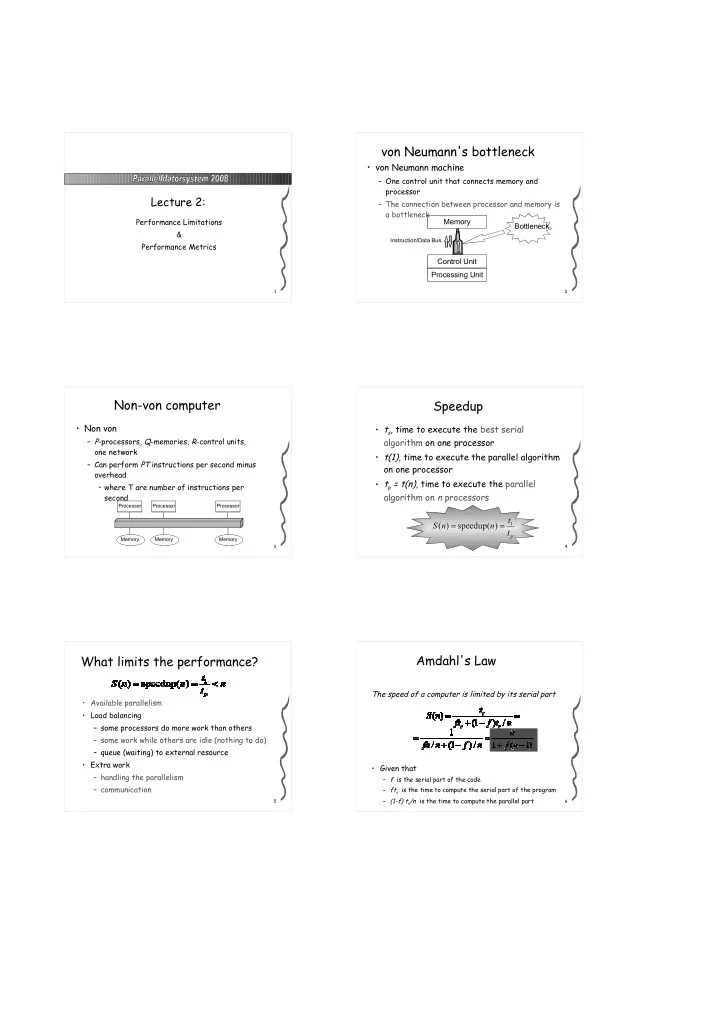
von Neumann's bottleneck • von Neumann machine – One control unit that connects memory and processor Lecture 2: – The connection between processor and memory is a bottleneck Performance Limitations Memory Bottleneck & Instruction/Data Bus Performance Metrics Control Unit Processing Unit 1 2 Non-von computer Speedup • Non von • t s , time to execute the best serial – P -processors, Q -memories, R -control units, algorithm on one processor one network • t(1) , time to execute the parallel algorithm – Can perform PT instructions per second minus on one processor overhead • t p = t(n) , time to execute the parallel • where T are number of instructions per algorithm on n processors second Processor Processor Processor t = = S ( n ) speedup( n ) 1 t p Memory Memory Memory 3 4 Amdahl's Law What limits the performance? The speed of a computer is limited by its serial part • Available parallelism • Load balancing – some processors do more work than others – some work while others are idle (nothing to do) – queue (waiting) to external resource • Extra work • Given that – handling the parallelism – f is the serial part of the code – communication – ft s is the time to compute the serial part of the program – (1-f) t s /n is the time to compute the parallel part 5 6

Gustavson-Barsis’ Law Amdahl's Law - implications The parallel fraction of the problem is scalable - 20 increases with problem size 16 f =0 • Observation, Amdahl's law make the assumption that 12 f =0,05 (1- f) is independent of n , which it in most cases are not S(n) • New Law: 8 f =0,1 f =0,2 4 • Assume that – Parallelism can be used to increase the parallel part of the 0 problem 1 2 3 4 5 6 7 8 9 10 11 12 13 14 15 16 17 18 19 20 n 7 8 – Each processor computes both a serial ( s ) and a parallel ( p ) part Gustavson-Barsis’ Law - The nature of Parallel Programs implications • Embarrassingly parallel – speedup(p)= p 20 – Matrix addition, compilation of independent f =0 subroutines 16 • Divide and Conquer f =0,2 12 – speedup(p) ~ p/log 2 p S(n) – Binary tree: adding p numbers, merge sort 8 • Communication bound parallelism 4 – cost = latency + n/bandwidth - overlap – May even be slower on more processors 0 1 2 3 4 5 6 7 8 9 10 11 12 13 14 15 16 17 18 19 20 n – Matrix computations where whole structures must 9 10 be communicated, parallel program on LAN. Some measures of performance Benchmark Performance • Number of floating point operations per second – flop/s, Mflop/s, Gflop/s, Tflop/s • Used to measure a system's capacity in • Speedup curves: x-axis #processors, y-axis speedup different aspects. – Speedup s = t 1 /t(p). In teory limited by the number of • For example floating point speed, I/O-speed, processors. speedup for some core routines, ... • Scaled Speedup – Increases the problem size linjearly with the #processors • Benchmark suite : A collection of special- • Other measures character-benchmarks – Time, Problem size, Processor usage • Synthetic benchmark : A small benchmark that – Efficiency – Scalability imitates a real application with respect to • Several users on the system data structures and number of statements. – Throughput, (Jobs/sec) 11 12

Classical Benchmarks Parallel Benchmarks • Whetstone (synthetic, numerical) • Linpack (LU), Performance numbers by • Dhrystone (synthetic, integer) solving of linear equation systems • Linpack (Solves a 100x100 system, Mflop/s ) • NAS Kernels (7 FORTRAN routins, • Gemm-based fluid dynamics) • Livermore Loops (a number of loops) • Livermore Loops (FORTRAN code) • Perfect Club • SLALOM (sci. comp., how much can be www.netlib.org och computed in one minute) www.netlib.org/benchmark/linpackjava 13 14 Benchmark using linear equation LINPACK 100 systems • Matrices of size 100 • No changes of the FORTRAN-code are • The result reflects – Performance by solving dense equation allowed systems • High percentage of floating point – Arithmetic in full precision operations • Four different values – Linpack benchmark for matrices of size 100 – routines: ( SD)GEFA & ( SD)GESL – TPP: Solves systems of the order of 1000 (no – LU with partial pivoting and backward restrictions on method or implementation) substitution – Theoretical peak performance • Column oriented algorithms – HPC: Highly parallel computing 15 16 LINPACK 1000 Theoretical peak performance (T ovards P eak P erformace ) • Number of flops that can be computed during a specified time • Matrices of size 1000 • Allowed to change and substitute algorithm and • Based on the cycle time of the machine software • Example: Cray Y-MP/8, cycle time 6ns – Must use the same driver program and have m (2 operations/1 cycle) * (1 cycle/6ns) = 333 the same result and accuracy Mflop/s – 2n 3 /3 + O(2n 2 ) operations • Example: POWER3-200, cycle time 5ns • Gives an upper limit of the performance m (2x2 operationer/1 cycle) * (1 cycle/5ns) = – “the manufacturer guaranties that programs will not exceed this speed” 800 Mflop/s 17 18

Highly Parallel Computing Top 500 Supercomputer sites • The result reflects the problem size • Rules • A lista with the 500 most powerful – Solve systems of linear equations computer systems – Allow the problem size to vary – Use 2n 3 /3 + O(2n 2 ) operations (independent of method) • The computers are ranked by their • Result LINPACK benchmark performance – R max : maximal measured performance in Gflops – N max : the size for that problem • The list shows R max , N max , N 1/2 , R peak , – N 1/2 : the size where half of R max is achieved #processors – R peak : theoretical peak performance m http://www.top500.org www.netlib.org/benchmark/hpl/ 19 20 NAS, The kernel benchmarks NAS parallel benchmark • Embarrassingly parallel • Imitates computations and data movements in – Performance without communication Computational fluid dynamics (CFD) • Multigrid – Five parallel kernels & three simulated application – Structured ”long-distance-communication” benchmarks • Conjugated gradient – The problems are algorithmically specified – Non structured ”long-distance-communication”, • Three classes of problem (the main diffence is unstructured matrix-vector-operations the problem size) • 3d fft – Sample code, Class A och Class B (in increasing size) – ”long-distance-communication” • Result • Integer sort – Time in seconds – Integer computations and communication – Compared to Cray Y-MP/1 21 22 Twelve Ways to Fool the Masses NAS, Simulated kernels • Quote 32-bit performance results and compare it with others 64-bit results • Present inner kernel performance figures as the • Pseudo-applications without the performance of entire application ”difficulties” existing in real CFD • Quietly employ assembly code and compare your results with others C or Fortran implementations – LU solver • Scale up the problem size with the number of processors – Pentadiagonal solver but fail to disclose this fact – Block-triangular solver • Quote performance results linearly projected to a full system • Compare with an old code on an obsolete system • Compare your results against scalar, un-optimized code on 23 Cray 24

Twelve Ways to Fool the Masses (2) Example of a perfomance graph • Base Mflop operation counts on the parallel Factorization on IBM POWER3 700 implementation, not on the best sequential algorithm 600 • Quote performance in terms of processor utilization, parallel speedup or Mflops/dollar (Peak not sustained) 500 • Measure parallel run time on a dedicated system but 400 Mflops/s measure conventional run times in a busy environment 300 • If all these fails, show pretty pictures and animated videos, and don’t talk about performance 200 D. H. Bailey, "Twelve Ways to Fool the Masses When Giving Performance Results on Parallel Computers," in Proceedings of Supercomputing '91 , Nov. 1991, pp. 4-7. 100 BC, without data transformation BC, including time for data transformation (finns bl a på www.pdc.kth.se/training/twelve-ways.html) LAPACK DPOTRF LAPACK DPPTRF 0 0 100 200 300 400 500 600 700 800 900 1000 N 25 26 Example of a performance graph Räkneuppgifter • Hur mycket speedup kan man få enligt Amdahl’s lag när n->stort? Applicera slutsatsen på ett program Factorization on IBM POWER2 450 med 5% seriell del! 400 • Vid en testkörning på en CPU tog ett program 30 350 sek för storlek n. För fyra CPU tog det 20 sek. Hur lång tid kräver samma program på 10 CPU enl. 300 Amdahl’s lag? Vad blir speedup? Hur lång tid enl. 250 Mflops/s Gustafson-Barsis’ lag för 10 n och 10 CPU? Vad blir 200 speedup? 150 • En parallelldator består av 16 CPU med vardera 800 MIPS topprestanda. Vad blir prestandan (i MIPS) 100 om de instruktioner som skall utföras är 10% seriell BPC, without data transformation 50 BPC, including time for data transformation LAPACK DPOTRF kod, 20% parallell för 2 CPU och 70% fullt LAPACK DPPTRF 0 27 28 0 100 200 300 400 500 600 700 800 900 1000 parallelliserbar? N Tentamen 040116, uppgift 1. • Vad är parallella beräkningar? • Vid design av parallella program är följande begrepp viktiga: datapartitionering, kornighet och lastbalans. Förklara dessa begrepp! • Beskriv Flynn’s klassindelning. Ge exempel på maskiner som hör till varje klass! 29