Visualizing Quadratics 16-385 Computer Vision (Kris Kitani) - - PowerPoint PPT Presentation

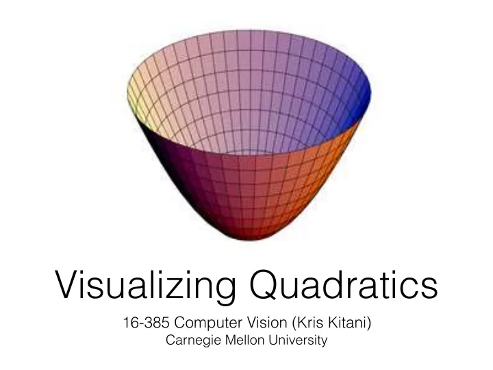
Visualizing Quadratics

16-385 Computer Vision (Kris Kitani)

Carnegie Mellon University

f(x, y) = x2 + y2 1 = x2 + y2 Equation of a circle Equation of a ‘bowl’ (paraboloid) If you slice the bowl at f(x, y) = 1 what do you get?

f(x, y) = x2 + y2 1 = x2 + y2 Equation of a circle Equation of a ‘bowl’ (paraboloid) If you slice the bowl at f(x, y) = 1 what do you get?

f(x, y) = x2 + y2

can be written in matrix form like this…

f(x, y) = ⇥ x y ⇤  1 1  x y

• 2.5
• 2
• 1.5
• 1
• 0.5

0.5 1 1.5 2 2.5

• 2
• 1.5
• 1
• 0.5

0.5 1 1.5 2

f(x, y) = ⇥ x y ⇤  1 1  x y

• ‘sliced at 1’

f(x, y) = ⇥ x y ⇤  2 1  x y

• What happens if you increase

coefficient on x?

and slice at 1

• 2.5
• 2
• 1.5
• 1
• 0.5

0.5 1 1.5 2 2.5

• 2
• 1.5
• 1
• 0.5

0.5 1 1.5 2

f(x, y) = ⇥ x y ⇤  2 1  x y

• What happens if you increase

coefficient on x?

and slice at 1

decrease width in x!

• 2.5
• 2
• 1.5
• 1
• 0.5

0.5 1 1.5 2 2.5

• 2
• 1.5
• 1
• 0.5

0.5 1 1.5 2

f(x, y) = ⇥ x y ⇤  2 1  x y

• What happens if you increase

coefficient on x?

and slice at 1

decrease width in x! What happens to the gradient in x? increases gradient in x ‘thins the bowl in x’

f(x, y) = ⇥ x y ⇤  1 2  x y

• What happens if you increase

coefficient on y?

and slice at 1

f(x, y) = ⇥ x y ⇤  1 2  x y

• What happens if you increase

coefficient on y?

and slice at 1

• 2.5
• 2
• 1.5
• 1
• 0.5

0.5 1 1.5 2 2.5

• 2
• 1.5
• 1
• 0.5

0.5 1 1.5 2

decrease width in y

f(x, y) = ⇥ x y ⇤  1 2  x y

• What happens if you increase

coefficient on y?

and slice at 1

• 2.5
• 2
• 1.5
• 1
• 0.5

0.5 1 1.5 2 2.5

• 2
• 1.5
• 1
• 0.5

0.5 1 1.5 2

decrease width in y What happens to the gradient in y?

f(x, y) = ⇥ x y ⇤  1 2  x y

• What happens if you increase

coefficient on y?

and slice at 1

• 2.5
• 2
• 1.5
• 1
• 0.5

0.5 1 1.5 2 2.5

• 2
• 1.5
• 1
• 0.5

0.5 1 1.5 2

decrease width in y What happens to the gradient in y? increases gradient in y ‘thins the bowl in y’

f(x, y) = x2 + y2 can be written in matrix form like this… f(x, y) = ⇥ x y ⇤  1 1  x y

• What’s the shape?

What are the eigenvectors? What are the eigenvalues?

f(x, y) = x2 + y2 can be written in matrix form like this… f(x, y) = ⇥ x y ⇤  1 1  x y

•  1

1

• =

 1 1  1 1  1 1 >

eigenvalues along diagonal eigenvectors

Result of Singular Value Decomposition (SVD)

axis of the ‘ellipse slice’ gradient of the quadratic along the axis

T

! " # $ % & ! " # $ % & ! " # $ % & = ! " # $ % & = 1 1 1 1 1 1 1 1 A

Eigenvalues Eigenvectors Eigenvectors

Eigenvector Eigenvector

x y x y

*not the size of the axis

f(x, y) = ⇥ x y ⇤  1 1  x y

• you can smash this bowl in the y direction

f(x, y) = ⇥ x y ⇤  1 4  x y

• you can smash this bowl in the x direction

f(x, y) = ⇥ x y ⇤  4 1  x y

• Recall:

T

! " # $ % & ! " # $ % & ! " # $ % & = ! " # $ % & = 1 1 1 4 1 1 1 4 A

Eigenvalues Eigenvectors Eigenvectors

Eigenvector Eigenvector

x y x y

*not the size of the axis (inverse relation)

T

! " # $ % & − − − ! " # $ % & ! " # $ % & − − − = ! " # $ % & = 50 . 87 . 87 . 50 . 4 1 50 . 87 . 87 . 50 . 75 . 1 30 . 1 30 . 1 25 . 3 A

Eigenvalues Eigenvectors Eigenvectors

Eigenvector Eigenvector

T

! " # $ % & − − − ! " # $ % & ! " # $ % & − − − = ! " # $ % & = 50 . 87 . 87 . 50 . 10 1 50 . 87 . 87 . 50 . 25 . 3 90 . 3 90 . 3 75 . 7 A

Eigenvalues Eigenvectors Eigenvectors

Eigenvector Eigenvector

Error function 


(for Harris corners)

The surface E(u,v) is locally approximated by a quadratic form

We will need this to understand…

Conic section of Error function

Since M is symmetric, we have

We can visualize M as an ellipse with axis lengths determined by the eigenvalues and orientation determined by R

direction of the slowest change (smaller gradient) direction of the fastest change (larger gradient)

(λmax)-1/2 (λmin)-1/2

Ellipse equation: ⇥ u v ⇤ M  u v

• = 1

‘isocontour’

but smaller axis

• n ‘slice’

but larger axis

• n ‘slice’