Virtual Inertia Emulation and Placement in Power Grids S eminaire - - PowerPoint PPT Presentation

SLIDE 1

Virtual Inertia Emulation and Placement in Power Grids

S´ eminaire d’Automatique du Plateau de Saclay Laboratoire de Signaux et Syst` emes du Supelec

Florian D¨

• rfler

At the beginning of power systems was . . .

At the beginning was the synchronous machine: M d dt ω(t) = Pgeneration(t) − Pdemand(t) change of kinetic energy = instantaneous power balance Fact: the AC grid & all of power system operation has been designed around synchronous machines.

Pgeneration Pdemand ω

2 / 35

Operation centered around bulk synchronous generation

49.88 49.89 49.90 49.91 49.92 49.93 49.94 49.95 49.96 49.97 49.98 49.99 50.00 50.01 50.02 16:45:00 16:50:00 16:55:00 17:00:00 17:05:00 17:10:00 17:15:00

• 8. Dezember 2004

f [Hz] 49.88 49.89 49.90 49.91 49.92 49.93 49.94 49.95 49.96 49.97 49.98 49.99 50.00 50.01 50.02 16:45:00 16:50:00 16:55:00 17:00:00 17:05:00 17:10:00 17:15:00

• 8. Dezember 2004

f [Hz]

Frequency Athens f - Setpoint Frequency Mettlen, Switzerland PP - Outage PS Oscillation

Source: W. Sattinger, Swissgrid Primary Control Secondary Control Tertiary Control Oscillation/Control Mechanical Inertia

3 / 35

Distributed/non-rotational/renewable generation on the rise

Source: Renewables 2014 Global Status Report

4 / 35

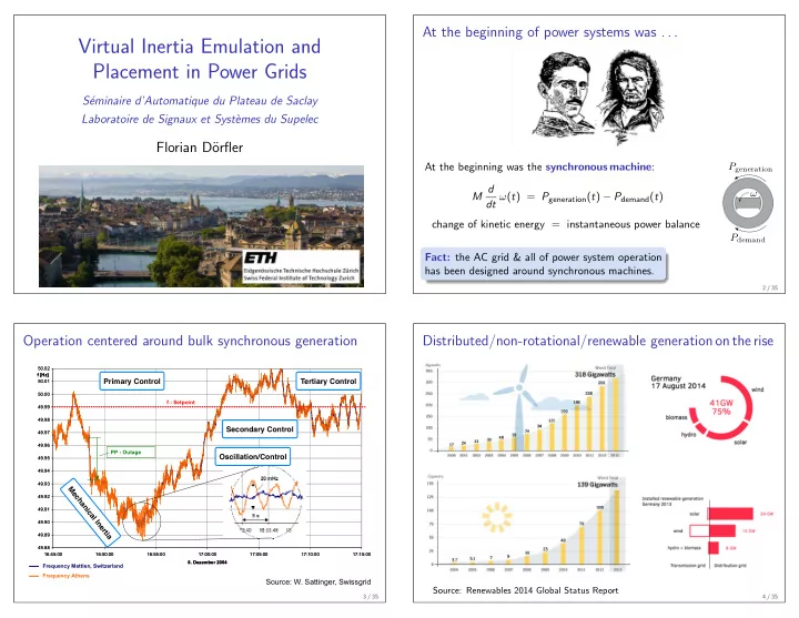
SLIDE 2

A few (of many) game changers . . .

synchronous generator new workhorse scaling location & distributed implementation

Almost all operational problems can principally be resolved . . . but one (?)

5 / 35

Fundamental challenge: operation of low-inertia systems

We slowly loose our giant electromechanical low-pass filter: M d dt ω(t) = Pgeneration(t) − Pdemand(t) change of kinetic energy = instantaneous power balance

Pgeneration Pdemand ω

6 / 35

Low-inertia stability: # 1 problem of distributed generation

# frequency violations in Nordic grid

(source: ENTSO-E)

15

Number * 10 5000 10000 15000 20000 25000 30000 Duration [s] Events [-] Months of the year Number * 10 Duration 2001 2002 2003 2004 2006 2005 2007 2008 2009 2010

it eal

same in Switzerland (source: Swissgrid) inertia is shrinking, time-varying, & localized, . . . & increasing disturbances Solutions in sight: none really . . . other than emulating virtual inertia through fly-wheels, batteries, super caps, HVDC, demand-response, . . .

7 / 35

Virtual inertia emulation

devices commercially available, required by grid-codes or incentivized through markets

!""" #$%&'%(#!)&' )& *)+"$ ','#"-'. /)01 23. &)1 2. -%, 2456 5676

!89:;8;<=><? />@=AB: !<;@=>B >< CD!EFGBH;I +><I *JK;@ E;<;@B=>J<

• JLB88BI@;MB DBNLB@> -J?LBIIB8 %@B<>! "#$%&'# (&)*&+! ,---. B<I "LBO D1 ":F'BBIB<P! "&'./+ (&)*&+! ,---

!"#$%&'"'() %* +$,(-.'() /'-#%(-' .( 0.1$%2$.3- 4-.(2 5.$)6,7 !('$).,

8.".-9 :%(.! "#$%&'# (&)*&+! ,---; :6$<,(,$,<,(, =%%77,! (&)*&+! ,---; ,(3 06>67 ?@ ?9,(3%$>,$! (&)*&+! ,---

Virtual synchronous generators: A survey and new perspectives

Hassan Bevrani a,b,⇑, Toshifumi Ise b, Yushi Miura b

a Dept. of Electrical and Computer Eng., University of Kurdistan, PO Box 416, Sanandaj, Iran b Dept. of Electrical, Electronic and Information Eng., Osaka University, Osaka, Japan

!"#$%&'()*+,-+#'"(./#0*/1(2-33/*04($(5&*0-$1(( 6#+*0&$(7*/8&9+9(:"(!&;0*&:-0+9(<#+*="(20/*$=+( 0/(6;/1$0+9(7/>+*(2";0+%;((

?$-0@&+*(!+1&11+A(!"#$"%&'()))A(B*-#/()*$#C/&;A(*"+,-%'!"#$"%&'()))A($#9(?&11+;(D$1$*$#=+(

!""" #$%&'%(#!)&' )& *)+"$ ','#"-'. /)01 23. &)1 2. -%, 2456

!789:;< "=>?<:;@7 (@7:9@? ':9<:8AB C@9 /'(DE/F( #9<7G=;GG;@7 'BG:8=G

H;8I8; JK>. (<=LI8?? F1 M@@:K. N9<;7 *1 %O<=. %7O98P H1 $@GQ@8. <7O (K9;G N1 M9;AK:

!"#$%&#'$%()*+'",'"%-#,.%/#",012%3#*',#4% 5,)"16'%

7898:%+1*%;'<'*=''4>?%@%58;8A8%$'%A11*?@%!"#$%&'("()"&*'+,,,@%98%/1"'21B%1*$%38%/#<<4.'"C@% !"#$%&'("()"&'+,,,%

M d dt ω(t) = Pgeneration(t)−Pdemand(t) . . . essentially D-control ⇒ plug-&-play (decentralized & passive), grid-friendly, user-friendly, . . . ⇒ today: where to do it? how to do it properly?

8 / 35

SLIDE 3

Outline

Introduction Novel Virtual Inertia Emulation Strategy Optimal Placement of Virtual Inertia Conclusions

inertia emulation

Classification & choice of actuators

(source: Stephan Masselis)

each of these (& far more) have been proposed for virtual inertia emulation

9 / 35

Inertia emulation & virtual synchronous machines

1 naive D-control on ω(t):

M d

dt ω(t) = Pgeneration(t) − Pdemand(t)

2 more sophisticated emulation of virtual synchronous machine Virtual synchronous generators: A survey and new perspectives

Hassan Bevrani a,b,⇑, Toshifumi Ise b, Yushi Miura b

a Dept. of Electrical and Computer Eng., University of Kurdistan, PO Box 416, Sanandaj, Iran b Dept. of Electrical, Electronic and Information Eng., Osaka University, Osaka, Japan

Contents lists available at ScienceDirect

Electrical Power and Energy Systems

journal homepage: www.elsevier.com/locate/ijepes

3 everything in between . . . and much more . . .

⇒ by measuring AC current/voltage/power/frequency ⇒ software model of virtual machine provides converter setpoints ⇒ actuation via modulation (switching) or DC injection (batteries etc.)

10 / 35

SLIDE 4

Challenges in real-world converter implementations

Virtual synchronous generators: A survey and new perspectives

Hassan Bevrani a,b,⇑, Toshifumi Ise b, Yushi Miura b

a Dept. of Electrical and Computer Eng., University of Kurdistan, PO Box 416, Sanandaj, Iran b Dept. of Electrical, Electronic and Information Eng., Osaka University, Osaka, Japan Contents lists available at ScienceDirect

Electrical Power and Energy Systems

journal homepage: www.elsevier.com/locate/ijepes

Abstract- The method to investigate the interaction between a Virtual Synchronous Generator (VSG) and a power system is presented here. A VSG is a power-electronics based device that To better study and witness the effects of virtual inertia, the hardware of a real VSG should be tested within a power

• system. Investigating the interaction between a real VSG and

a power system is not easy as a power system cannot be

Real Time Simulation of a Power System with VSG Hardware in the Loop

Vasileios Karapanos, Sjoerd de Haan, Member, IEEE, Kasper Zwetsloot Faculty of Electrical Engineering, Mathematics and Computer Science Delft University of Technology Delft, the Netherlands E-mails: vkarapanos@gmail.com, v.karapanos@tudelft.nl, s.w.h.dehaan@tudelft.nl

• 1 delays in measurement acquisition, signal processing, & actuation

2 accuracy in AC measurements (averaged over ≈ 5 cycles) 3 constraints on currents, voltages, power, etc. 4 guarantees on stability and robustness

today: use DC measurement, exploit analog storage, & passive control

11 / 35

Averaged inverter model

iload

−

+ vx iαβ R L ic C

+

− vαβ idc Gdc Cdc ix

DC cap & AC filter equations:

Cdc ˙ vdc = −Gdcvdc + idc − 1 2m⊤iαβ C ˙ vαβ = −iload + iαβ L ˙ iαβ = −Riαβ + 1 2mvdc − vαβ

modulation: ix = 1

2m⊤iαβ , vx = 1 2mvdc

passive: (idc, iload)→(vdc, vαβ) model of a synchronous generator

˙ θ = ω M ˙ ω = −Dω + τm + i⊤

αβLmif

− sin(θ) cos(θ)

• C ˙

vαβ = −Gloadvαβ + iαβ Ls ˙ iαβ = −Riαβ − vαβ − ωLmif − sin(θ) cos(θ)

• if

θ

12 / 35

standard power electronics control would continue by

1 constructing voltage/current/power references

(e..g, droop, synchronous machine emulation, etc.)

2 tracking these references at the converter terminals

typically by means of cascaded PI controllers let’s do something different (smarter?) today . . .

13 / 35

See the similarities & the differences ?

iload

−

+ vx iαβ R L ic C

+

− vαβ idc Gdc Cdc ix

DC cap & AC filter equations:

Cdc ˙ vdc = −Gdcvdc + idc − 1 2m⊤iαβ C ˙ vαβ = −iload + iαβ L ˙ iαβ = −Riαβ + 1 2mvdc − vαβ

modulation: ix = 1

2m⊤iαβ , vx = 1 2mvdc

passive: (idc, iload)→(vdc, vαβ) model of a synchronous generator

˙ θ = ω M ˙ ω = −Dω + τm + i⊤

αβLmif

− sin(θ) cos(θ)

• C ˙

vαβ = −Gloadvαβ + iαβ Ls ˙ iαβ = −Riαβ − vαβ − ωLmif − sin(θ) cos(θ)

• if

θ

14 / 35

SLIDE 5

Model matching (= emulation) as inner control loop

iload

−

+ vx iαβ R L ic C

+

− vαβ idc Gdc Cdc ix

DC cap & AC filter equations:

Cdc ˙ vdc = −Gdcvdc + idc − 1 2m⊤iαβ C ˙ vαβ = −iload + iαβ L ˙ iαβ = −Riαβ + 1 2mvdc − vαβ

matching control: ˙

θ = η · vdc , m = µ ·

• − sin(θ)

cos(θ)

• with η, µ > 0

⇒ pros: is balanced, uses natural storage, & based on DC measurement ⇒ virtual machine with M = Cdc

η2 , D = Gdc η2 , τm = idc η , if = µ ηLm

⇒ base for outer controls via idc & µ, e.g., virtual torque, PSS, & inertia

15 / 35

Some properties & different viewpoints

1 quadratic curves for

stationary P vs. (|V |, ω) ⇒ P ≤ Pmax = i2

dc/4Gdc

⇒ reactive power not directly affected ⇒ (P, ω)-droop ≈ 1/η ⇒ (P, |V |)-droop ≈ 1/µ

2 reformulation as virtual

& adaptive oscillator

3 remains passive:

(idc, iload)→(vdc, vαβ)

0.5 1 1.5 2

Active power P

×104 50 100 150 200

Amplitude (V)

Cdc ˙ vdc = −Gdcvdc + i∗

dc − 1

2m⊤iαβ C ˙ vαβ = −iload + iαβ L ˙ iαβ = −Riαβ + 1 2mvdc − vαβ ˙ ξ = vdcη · 1 −1

• ξ

η µ _ m vdc (idc, iload) (vdc, vαβ) inverter modulation

16 / 35

Eye candy: response to a load step

0.1 0.2 0.3 0.4 0.5 0.6 0.7 0.8 0.9 1

time(s)

0.05 0.1 0.15 0.2

gload(Ω-1)

0.1 0.2 0.3 0.4 0.5 0.6 0.7 0.8 0.9 1

time(s)

• 200
• 100

100 200

Vx Gload iload

−

+ vx iαβ R L ic C

+

− vαβ idc Gdc Cdc ix

0.1 0.2 0.3 0.4 0.5 0.6 0.7 0.8 0.9 1 time(s) 150 155 160 165 170 Amplitude (V) 0.1 0.2 0.3 0.4 0.5 0.6 0.7 0.8 0.9 1 time(s) 40 42 44 46 48 50 Frequency (Hz)

17 / 35

• ptimal placement
• f virtual inertia

SLIDE 6

Linearized & Kron-reduced swing equation model

mi ¨ θi + di ˙ θi = pin,i − pe,i generator swing equations pe,i ≈

j∈N bij(θi − θj)

linearized power flows likelihood of disturbance at #i: ti ≥ 0

ω

Pgeneration + η Pdemand

state space representation: ˙ θ ˙ ω

• =
• I

−M−1L −M−1D

• A

θ ω

• +
• M−1
• T 1/2
• B

η where M = diag(mi), D = diag(di), T = diag(ti), & L = LT (Laplacian)

18 / 35

Performance metric for emulation of rotational inertia

f restoration time nominal frequency max deviation effort ROCOF

System norm: amplification of disturbances: impulse (fault), step (loss of unit), white noise (renewables) to performance outputs: integral, peak, ROCOF, restoration time, . . .

19 / 35

Coherency performance metric & H2 norm

Energy expended by the system to return to synchronous operation: ∞

• {i, j}∈ Eaij(θi(t) − θj(t))2 +

n

i=1si ω2 i (t) dt

H2 norm interpretation:

1 associated performance output:

y =

• Q1/2

1

Q1/2

2

θ ω

• 2 impulses (faults) −

→ output energy ∞

0 y(t)T y(t) dt

3 white noise (renewables) −

→ output variance lim

t→∞ E

• y(t)T y(t)
• 20 / 35

Algebraic characterization of the H2 norm

Lemma: via observability Gramian

G2

2 = Trace(BTPB)

where P is the observability Gramian P = ∞

0 eATtC TCeAt dt ◮ P solves a Lyapunov equation: P A + ATP + Q = 0 ◮ A has a zero eigenvalue → restricts choice of Q

y =

• Q1/2

1

Q1/2

2

θ ω

• Q1/2

1

1 = 0

◮ P is unique for P [1 0] = [0 0]

21 / 35

SLIDE 7

Problem formulation

minimize

P , mi

G2

2 = Trace(BTPB)

→ performance metric subject to n

i=1 mi ≤ mbdg

→ budget constraint mi ≤ mi ≤ mi , i ∈ {1, . . . , n} → capacity constraint P A + ATP + Q = 0 → observability Gramian P [1 0] = [0 0] → uniqueness Insights

1 m appears as m−1 in system matrices A , B 2 product of B(m) & P in the objective 3 product of A(m) & P in the constraint

       ⇒ large-scale & non-convex

22 / 35

Building the intuition: results for two-area networks

Fundamental learnings

1 explicit closed-form solution is rational function 2 sufficiently uniform (t/d)i → strongly convex & fairly flat cost 3 non trivial in the presence of capacity constraints m1 2 4 6 8 10 f(m1) 1 2 3 4 5 6 dissimilar t/d identical t/d

Dissimilar and Identical t/d ratios

performance metric

t1=1-t2 0.1 0.2 0.3 0.4 0.5 0.6 0.7 0.8 0.9 1 Optimal inertia allocation 5 10 15 20 25 m1∗ m2∗ mbdg m1∗ + m2∗

Budget, Sum, Inertia1, Inertia2

• ptimal inertia allocation

23 / 35

Closed-form results for cost of primary control

P/ ˙ θ primary droop control

(ωi − ω∗) ∝ (Pi ∗ − Pi(θ))

• Di ˙

θi = Pi ∗ − Pi(θ)

P2 P1 P 𝜕 𝜕* 𝜕sync

Primary control effort → accounted for by integral quadratic cost ∞ ˙ θ(t)TD ˙ θ(t) dt which is the H2 performance for the penalties Q1/2

1

= 0 and Q1/2

2

= D

24 / 35

Primary Control . . . cont’d

Theorem: the primary control effort optimization reads equivalently as minimize

mi

n

i=1

ti mi subject to n

i=1 mi ≤ mbdg

mi ≤ mi ≤ mi, i ∈ {1, . . . , n} Key take-aways:

◮ optimal solution independent of network topology ◮ allocation ∝ √ti or mi = min{mbdg, mi}

Location & strength of disturbance are crucial solution ingredients

25 / 35

SLIDE 8

numerical method for the general case

Taylor & power series expansions

Key idea: expand the performance metric as a power series in m G2

2 = Trace(B(m)TP(m)B(m))

Motivation: scalar series expansion at mi in direction µi: 1 (mi + δµi) = 1 mi − δµi m2

i

+ O(δ2) Expand system matrices as Taylor series in direction µ: A(m + δµ) = A(0)

(m,µ) + A(1) (m,µ)δ + O(δ2)

B(m + δµ) = B(0)

(m,µ) + B(1) (m,µ)δ + O(δ2)

Expand the observability Gramian as a power series in direction µ: P(m + δµ) = P(0)

(m,µ) + P(1) (m,µ)δ + O(δ2)

26 / 35

Explicit gradient computation

Expansion of system matrices & Gramian ⇒ match coefficients . . .

Formula for gradient at m in direction µ

1 nominal Lyapunov equation for O(δ0):

P(0) = Lyap(A(0) , Q)

2 perturbed Lyapunov equation for O(δ1) terms:

P(1) = Lyap(A(0) , P(0)A(1) + A(1)TP(0))

3 expand objective in direction µ:

G2

2 = Trace(B(m)TP(m)B(m)) = Trace((. . .) + δ(. . .)) + O(δ2)

4 gradient: Trace(2 ∗ B(1)TP(0)B(0) + B(0)TP(1)B(0))

⇒ use favorite method for reduced optimization problem

27 / 35

results

SLIDE 9

Modified Kundur case study: 3 regions & 12 buses

transformer reactance 0.15 p.u., line impedance (0.0001+0.001i) p.u./km

10 9 5 1 11 12 7 6 3 4 2 8

28 / 35

Heuristics outperformed by H2 - optimal allocation

Scenario: disturbance at #4

◮ locally optimal solution

• utperforms heuristic

max/uniform allocation

◮ optimal allocation ≈

matches disturbance

◮ inertia emulation at all

undisturbed nodes is actually detrimental ⇒ location of disturbance & inertia emulation matters

node 1 2 4 5 6 8 9 10 12 inertia 40 80 120 160 m m∗ m trace 0.05 0.1 0.15 0.2 0.25 Cost

Original, Optimal, and Capacity allocations

allocation subject to capacity constraints

node 1 2 4 5 6 8 9 10 12 inertia 40 80 120 160 m m∗ muni trace 0.05 0.1 0.15 0.2 0.25

Cost Original, Optimal, and Uniform allocations

allocation subject to the budget constraint

29 / 35

Eye candy: time-domain plots of post fault behavior

Time(s) 50 100 150 ∆θ1-∆θ4

• 0.05
• 0.04
• 0.03
• 0.02
• 0.01

0.01 0.02 0.03 0.04 0.05 (a) Time(s) 50 100 150 ∆ω4

• 0.1
• 0.05

0.05 0.1 0.15 (b) Time(s) 50 100 150 ∆ω5 ×10-3

• 2
• 1

1 2 3 4 5 (c) Time(s) 50 100 150 Control effort

• 2.5
• 2
• 1.5
• 1
• 0.5

0.5 1 1.5 2 (d) m muni m∗

Control Effort Angle Diff. Freq #4 Freq #5 Original, Optimal, and Uniform allocations

Take-home messages:

best oscillation performance smallest peak frequency at #4 undisturbed sites are irrelevant minimal control effort mi · ¨ θi

30 / 35

conclusions

SLIDE 10

Conclusions on virtual inertia emulation

Where to do it?

1 H2-optimal (non-convex) allocation 2 closed-form results for cost of primary control 3 numerical approach via gradient computation

How to do it?

1 down-sides of naive inertia emulation 2 novel machine matching control

What else to do? Inertia emulation is . . .

decentralized, plug-and-play (passive), grid-friendly, user-friendly, . . . suboptimal, wasteful in control effort, & need for new actuators

31 / 35

Recall: operation centered around (virtual) sync generators

49.88 49.89 49.90 49.91 49.92 49.93 49.94 49.95 49.96 49.97 49.98 49.99 50.00 50.01 50.02 16:45:00 16:50:00 16:55:00 17:00:00 17:05:00 17:10:00 17:15:00

• 8. Dezember 2004

f [Hz] 49.88 49.89 49.90 49.91 49.92 49.93 49.94 49.95 49.96 49.97 49.98 49.99 50.00 50.01 50.02 16:45:00 16:50:00 16:55:00 17:00:00 17:05:00 17:10:00 17:15:00

• 8. Dezember 2004

f [Hz]

Frequency Athens f - Setpoint Frequency Mettlen, Switzerland PP - Outage PS Oscillation

Source: W. Sattinger, Swissgrid Primary Control Secondary Control Tertiary Control Oscillation/Control Inertia & Emulation

32 / 35

A control perspective of power system operation

Conventional strategy: emulate generator physics & control

M ˙ ω(t)

(virtual) inertia

= Pmech

tertiary control

− Dω(t)

primary control

− t ω(τ) d τ

• secondary control

− Pelec

Essentially all PID + setpoint control (simple, robust, & scalable)

M ˙ ω(t)

D

= P

• set-point

− Dω(t)

P

− t ω(τ) d τ

• I

− Pelec

Control engineers should be able to do better . . .

33 / 35

This “ what else? ” has been broadly recognized

by TSOs, device manufacturers, academia, etc.

Massive InteGRATion of power Electronic devices “The question that has to be examined is: how much power electronics can the grid cope with?” (European Commission) current controls what else? all options are on the table and keep us busy . . .

34 / 35

SLIDE 11

Acknowledgements

Taouba Jouini Catalin Arghir Dominic Gross Bala K. Poolla Saverio Bolognani

35 / 35

appendix

Spectral perspective on different inertia allocations

Real Axis

• 0.18
• 0.16
• 0.14
• 0.12
• 0.1
• 0.08
• 0.06
• 0.04
• 0.02

0.02

Imaginary Axis

• 3
• 2
• 1

1 2 3 cone m muni m∗

Cone, Original, Optimal, and Uniform allocations

• m = m → best damping asymptote & best damping ratio
• Spectrum holds only partial information !!

The planning problem

sparse allocation of limited resources

ℓ1-regularized inertia allocation (promoting a sparse solution): minimize

P , mi

Jγ(m, P) = G2

2 + γm − m1

subject to n

i=1 mi ≤ mbdg

mi ≤ mi ≤ mi i ∈ {1, . . . , n} P A + ATP + Q = 0 P[1 0] = [0 0] where γ ≥ 0 trades off sparsity penalty and the original objective Highlights:

1 regularization term is linear & differentiable 2 gradient computation algorithm can be used with some tweaking

SLIDE 12

Relative performance loss (%) as a function of γ

0% → optimal allocation, 100% → no additional allocation

γ

×10-4 0.5 1 1.5 2 2.5 3

Cardinality

2 4 6 8 10

Cardinality-Loc Cardinality-Uni Performance-Loc Performance-Uni

Relative Performance Loss (%)

20 40 60 80 100 20 40 60 80 100

Localized and Uniform disturbances

Card

• Perf. %

1 uniform disturbance ⇒ ∃ γ 1.3% loss ≡ (9 → 7) 2 localized disturbance ⇒ (2 → 1) without affecting performance

Uniform disturbance to damping ratio

power sharing → d ∝ P∗, assuming t ∝ source rating P∗

Theorem: for ti/di = tj/dj the allocation problem reads equivalently as minimize

mi

n

i=1

si mi subject to n

i=1 mi ≤ mbdg

mi ≤ mi ≤ mi, i ∈ {1, . . . , n} Key takeaways:

• ptimal solution independent of network topology

allocation ∝ √si or mi = min{mbdg, mi} What if freq. penalty ∝ inertia? → norm independent of inertia

Taylor & power series expansions

Key idea: expand the performance metric as a power series in m G2

2 = Trace(B(m)TP(m)B(m))

Motivation: scalar series expansion at mi in direction µi: 1 (mi + δµi) = 1 mi − δµi m2

i

+ O(δ2) Expand system matrices in direction µ, where Φ = diag(µ): A(0)

(m,µ) =

• I

−M−1L −M−1D

• , A(1)

(m,µ) =

• ΦM−2L

ΦM−2D

• B(0)

(m,µ) =

• M−1T 1/2
• , B(1)

(m,µ) =

• −ΦM−2T 1/2
• Taylor & power series expansions cont’d

Expand the observability Gramian as a power series in direction µ P(m) = P(m + δµ) = P(0)

(m,µ) + P(1) (m,µ)δ + O(δ2)

Formula for gradient in direction µ

1 nominal Lyapunov equation for O(δ0): P(0) = Lyap(A(0) , Q) 2 perturbed Lyapunov equation for O(δ1) terms:

P(1) = Lyap(A(0) , P(0)A(1) + A(1)TP(0))

3 expand objective in direction µ:

G2

2 = Trace(B(m)TP(m)B(m)) = Trace((. . .) + δ(. . .)) + O(δ2)

4 gradient: Trace(2 ∗ B(1)TP(0)B(0) + B(0)TP(1)B(0))

SLIDE 13

Gradient computation

Algorithm: Gradient computation & perturbation analysis Input → current values of the decision variables mi Output → numerically evaluated gradient ∇f of the cost function

1 Evaluate the system matrices A(0) , B(0) based on current inertia 2 Solve for P(0)=Lyap(A(0) , Q) using a Lyapunov routine 3 For each node- obtain the perturbed system matrices A(1) , B(1) 4 Compute P(1)=Lyap(A(0) , P(0)A(1) + A(1)TP(0)) 5 Gradient ⇒ Trace(2 ∗ B(1)TP(0)B(0) + B(0)TP(1)B(0))

Heuristics outperformed also for uniform disturbance

Cost Original, Optimal, and Capacity allocations

node 1 2 4 5 6 8 9 10 12 inertia 50 100 150 m m∗ m trace 0.05 0.1 0.15

allocation subject to capacity constraints

node 1 2 4 5 6 8 9 10 12 inertia 30 60 90 trace 0.05 0.1 0.15 m m∗ muni

Cost Original, Optimal, and Uniform allocations

allocation subject to the budget constraint

Scenario: uniform disturbance Heuristics for placement:

1 max allocation in case of

capacity constraints

2 uniform allocation in case

• f budget constraint

Results & insights:

1 locally optimal solution

• utperforms heuristics

2 optimal solution = max

inertia at each bus