
SLIDE 1
Practical Problems in VLSI Physical Design TimberWolf Placement (1/16)
TimberWolf 7.0 Placement
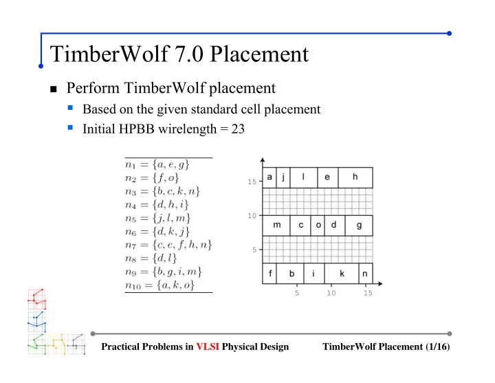
Perform TimberWolf placement
TimberWolf 7.0 Placement Perform TimberWolf placement Based on the - - PowerPoint PPT Presentation
TimberWolf 7.0 Placement Perform TimberWolf placement Based on the given standard cell placement Initial HPBB wirelength = 23 Practical Problems in VLSI Physical Design TimberWolf Placement (1/16) First Swap Swap node b and e
Practical Problems in VLSI Physical Design TimberWolf Placement (1/16)
Perform TimberWolf placement
Practical Problems in VLSI Physical Design TimberWolf Placement (2/16)
Swap node b and e
Practical Problems in VLSI Physical Design TimberWolf Placement (3/16)
ΔW = wirelength change from swap
Practical Problems in VLSI Physical Design TimberWolf Placement (4/16)
ΔWs = wirelength change from shifting
Practical Problems in VLSI Physical Design TimberWolf Placement (5/16)
Practical Problems in VLSI Physical Design TimberWolf Placement (6/16)
How accurate is ΔWs estimation?
Practical Problems in VLSI Physical Design TimberWolf Placement (7/16)
Based on piecewise linear graph
Practical Problems in VLSI Physical Design TimberWolf Placement (8/16)
Swap node m and o
Practical Problems in VLSI Physical Design TimberWolf Placement (9/16)
ΔW = wirelength change from swap
Practical Problems in VLSI Physical Design TimberWolf Placement (10/16)
Cell d and g are shifted
Practical Problems in VLSI Physical Design TimberWolf Placement (11/16)
Cell d and g are shifted
Practical Problems in VLSI Physical Design TimberWolf Placement (12/16)
Practical Problems in VLSI Physical Design TimberWolf Placement (13/16)
Swap node k and m
Practical Problems in VLSI Physical Design TimberWolf Placement (14/16)
ΔW = wirelength change from swap
Practical Problems in VLSI Physical Design TimberWolf Placement (15/16)
Cell c is shifted
Practical Problems in VLSI Physical Design TimberWolf Placement (16/16)