Very Large Scale Neighborhoods Weighted Matching Neighborhoods - PowerPoint PPT Presentation

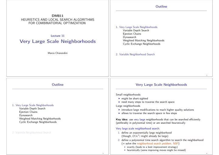
Outline DM811 HEURISTICS AND LOCAL SEARCH ALGORITHMS FOR COMBINATORIAL OPTIMZATION 1. Very Large Scale Neighborhoods Variable Depth Search Ejection Chains Lecture 11 Dynasearch Very Large Scale Neighborhoods Weighted Matching Neighborhoods Cyclic Exchange Neighborhoods Marco Chiarandini 2. Variable Neighborhood Search 2 Outline Very Large Scale Neighborhoods Small neighborhoods: ◮ might be short-sighted ◮ need many steps to traverse the search space 1. Very Large Scale Neighborhoods Large neighborhoods Variable Depth Search ◮ introduce large modifications to reach higher quality solutions Ejection Chains ◮ allows to traverse the search space in few steps Dynasearch Weighted Matching Neighborhoods Key idea: use very large neighborhoods that can be searched efficiently Cyclic Exchange Neighborhoods (preferably in polynomial time) or are searched heuristically Very large scale neighborhood search: 2. Variable Neighborhood Search 1. define an exponentially large neighborhood (though, O ( n 3 ) might already be large) 2. define a polynomial time search algorithm to search the neighborhood (= solve the neighborhood search problem, NSP) ◮ exactly (leads to a best improvement strategy) ◮ heuristically (some improving moves might be missed) 3 4

Variable Depth Search Examples of VLSN Search [Ahuja, Ergun, Orlin, Punnen, 2002]: ◮ based on concatenation of simple moves ◮ Key idea: Complex steps in large neighborhoods = variable-length ◮ Variable Depth Search (TSP, GP) sequences of simple steps in small neighborhood. ◮ Ejection Chains ◮ Use various feasibility restrictions on selection of simple search steps to ◮ based on Dynamic Programming or Network Flows limit time complexity of constructing complex steps. ◮ Dynasearch (ex. SMTWTP) ◮ Weighted Matching based neighborhoods (ex. TSP) ◮ Perform Iterative Improvement w.r.t. complex steps. ◮ Cyclic exchange neighborhood (ex. VRP) ◮ Shortest path ◮ based on polynomially solvable special cases of hard combinatorial Variable Depth Search (VDS): optimization problems determine initial candidate solution s ◮ Pyramidal tours ^ t := s ◮ Halin Graphs while s is not locally optimal do repeat ➤ ⇒ Idea: turn a special case into a neighborhood select best feasible neighbor t VLSN allows to use the literature on polynomial time algorithms if g ( t ) < g (^ t ) then ^ t := t s := ^ t until construction of complex step has been completed ; 5 7 VLSN for the Traveling Salesman Problem The Lin-Kernighan (LK) Algorithm for the TSP (1) ◮ k -exchange heuristics ◮ Complex search steps correspond to sequences ◮ 2-opt [Flood, 1956, Croes, 1958] of 2-exchange steps and are constructed from ◮ 2.5-opt or 2H-opt sequences of Hamiltonian paths ◮ Or-opt [Or, 1976] ◮ 3-opt [Block, 1958] ◮ δ -path: Hamiltonian path p + 1 edge connecting one end of p to ◮ k -opt [Lin 1965] interior node of p ◮ complex neighborhoods u v ◮ Lin-Kernighan [Lin and Kernighan, 1965] ◮ Helsgaun’s Lin-Kernighan a) ◮ Dynasearch u w v ◮ Ejection chains approach b) 8 9

Basic LK exchange step: ◮ Start with Hamiltonian path ( u, . . . , v ) : Construction of complex LK steps: u v 1. start with current candidate solution (Hamiltonian cycle) s ; set t ∗ := s ; a) set p := s ◮ Obtain δ -path by adding an edge ( v, w ) : 2. obtain δ -path p ′ by replacing one edge in p u v w 3. consider Hamiltonian cycle t obtained from p by b) (uniquely) defined edge exchange ◮ Break cycle by removing edge ( w, v ′ ) : 4. if w ( t ) < w ( t ∗ ) then set t ∗ := t ; p := p ′ ; go to step 2 u w v' v else accept t ∗ as new current candidate solution s c) ◮ Note: Hamiltonian path can be completed into Hamiltonian cycle by adding edge ( v ′ , u ) : Note: This can be interpreted as sequence of 1-exchange steps that alternate between δ -paths and Hamiltonian cycles. u w v' v c) 10 11 Additional mechanisms used by LK algorithm: Elements for an efficient neighborhood search ◮ Pruning exact rule: If a sequence of numbers has a positive sum, there is a cyclic permutation of these numbers such that every partial sum is positive. ➨ need to consider only gains whose partial sum remains positive ◮ fast delta evaluations ◮ Tabu restriction: Any edge that has been added cannot be removed and any edge that has been removed cannot be added in the same LK step. ◮ neighborhood pruning: fixed radius nearest neighborhood search Note: This limits the number of simple steps in a complex LK step. ◮ neighborhood lists: restrict exchanges to most interesting candidates ◮ Limited form of backtracking ensures that local minimum found by the algorithm is optimal w.r.t. standard 3-exchange neighborhood ◮ don’t look bits: focus perturbative search to “interesting” part ◮ (For further details, see original article) ◮ sophisticated data structures for fast updates [LKH Helsgaun’s implementation http://www.akira.ruc.dk/~keld/research/LKH/ (99 pages report)] 12 13

TSP data structures Ejection Chains Static data structures: ◮ Attempt to use large neighborhoods without examining them ◮ priority lists exhaustively ◮ k-d trees ◮ Sequences of successive steps each influenced by the precedent and determined by myopic choices Tour representation. Operations needed: ◮ Limited in length ◮ reverse ( a, b ) ◮ succ ( a ) ◮ Local optimality in the large neighborhood is not guaranteed. ◮ prec ( a ) Example (on TSP) : ◮ sequence(a,b,c) – check whether b is within a and b successive 2-exchanges where each exchange involves one edge of the Possible choices (dynamic data structure): previous exchange ◮ | V | < 1.000 arries π and π − 1 Example (on GCP) : ◮ | V | < 1.000.000 two level tree successive 1-exchanges: a vertex v 1 changes color from ϕ ( v 1 ) = c 1 to c 2 , in turn forcing some vertex v 2 with color ϕ ( v 2 ) = c 2 to change to another color ◮ | V | > 1.000.000 splay tree c 3 (which may be different or equal to c 1 ) and again forcing a vertex v 3 with color ϕ ( v 3 ) = c 3 to change to color c 4 . 14 16 Dynasearch Weighted Matching Neighborhoods ◮ Iterative improvement method based on building complex search steps from combinations of mutually independent search steps ◮ Mutually independent search steps do not interfere with each other w.r.t. effect on evaluation function and feasibility of candidate solutions. ◮ Key idea use basic polynomial time algorithms, example: weighted matching in bipartied graphs, shortest path, minimum spanning tree. Example: Independent 2-exchange steps for the TSP: ◮ Neighborhood defined by finding a minimum cost matching on a (non-)bipartite improvement graph u 1 u i u i+1 u j u j+1 u k u k+1 u l u l+1 u n u n+1 Example (TSP) Therefore: Overall effect of complex search step = sum of effects of Neighborhood: Eject k nodes and reinsert them optimally constituting simple steps; complex search steps maintain feasibility of candidate solutions. ◮ Key idea: Efficiently find optimal combination of mutually independent simple search steps using Dynamic Programming . 18 20

Cyclic Exchange Neighborhoods ◮ Possible for problems where solution can be represented as form of partitioning Neighborhood search ◮ Definition of a partitioning problem: Given: a set W of n elements, a collection T = { T 1 , T 2 , . . . , T k } of ◮ Define an improvement graph subsets of W , such that W = T 1 ∪ . . . ∪ T k and T i ∩ T j = ∅ , and a cost function c : T → R : Task: Find another partition T ′ of W by means of single exchanges ◮ Solve the relative between the sets such that ◮ Subset Disjoint Negative Cost Cycle Problem k � min c ( T i ) ◮ Subset Disjoint Minimum Cost Cycle Problem i = 1 ◮ Cyclic exchange: 22 23 Example (GCP) Example (GCP) Exponential size but can be searched efficiently One Exchange Path Exchange Improvement Graph A Subset Disjoint Negative Cost Cycle Problem in the Improvement Graph can be solved by dynamic programming in O ( | V | 2 2 k | D ′ | ) . Swap Cyclic Exchange Yet, heuristics rules can be adopted to reduce the complexity to O ( | V ′ | 2 ) 24 25