Vectors, matrices, eigenvalues and eigenvectors 1 1 2 0 . 5 2 - PowerPoint PPT Presentation

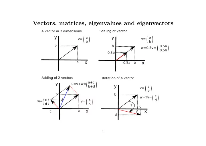
Vectors, matrices, eigenvalues and eigenvectors 1

� 1 � 2 � � 0 . 5 × 2 � � Scaling a vector: 0 . 5 � V = 0 . 5 = = 1 0 . 5 × 1 0 . 5 � 2 � � 1 � � 2 + 1 � � 3 � Adding two vectors: � V + � W = + = = 1 3 1 + 3 4 � a b � � λa λb � A scalar times a matrix: λ = c d λc λd � a b � � x y � � a + x b + y � A matrix plus a matrix: + = c d z w c + z d + w � a b � � x y � � ax + bz ay + bw � A matrix times a matrix: = c d z w cx + dz cy + dw 2

Hence the product of a matrix times a vector: � a b � � x � � ax + by � = c d y cx + dy This matrix transforms the vector into another vector: 3

4

� x − 2 y = − 5 A system of linear equations: 2 x + y = 10 � 1 − 2 � � x � � − 5 � Can be written as: = 2 1 y 10 From the first we obtain x = 2 y − 5, which gives in the second: 2(2 y − 5)+ y = 10 or 4 y − 10+ y = 10 or 5 y = 20 i.e. y = 4 , and hence x = 3. � a b � Finally, for the matrix A = define c d det[ A ] = ad − bc and tr[ A ] = a + d for the determinant and the trace. 5

Linear systems only have solutions when det[ A ] � = 0. Consider the following general linear system � ax + by = p cx + dy = q . Solve x = p a − by a from first equation, then: cp a − cby a + dy = q or cp − cby + ady = qa or y = qa − cp y ( ad − cb ) = qa − cp or ad − cb , which only has a finite solution when the denominator ad − cb is not equal to zero. 6

Forest succession: Gray Birch Blackgum Red Maple Beech Gray Birch 0.05 0.01 0 0 Blackgum 0.36 0.57 0.14 0.01 Red Maple 0.5 0.25 0.55 0.03 Beech 0.09 0.17 0.31 0.96 For example, the fraction of Red Maple trees after 50 years would be 0 . 5 × the fraction of Gray Birch trees, plus 0 . 25 × the fraction of Blackgum trees, plus 0 . 55 × the fraction of Red Maples, plus 0 . 03 × the fraction of Beech trees. 7

Write table as a matrix:   0 . 05 0 . 01 0 0 0 . 36 0 . 57 0 . 14 0 . 01   A =   0 . 5 0 . 25 0 . 55 0 . 03   0 . 09 0 . 17 0 . 31 0 . 96 and define the current state of the forest as a vector, e.g., � � � V 0 = 1 0 0 0 After 50 years the next state of the forest is defined by: V 50 = A � � � � V 0 = 0 . 05 0 . 36 0 . 5 0 . 09 which is a forest with 5% Gray Birch, 36% Blackgum, 50% Red Maple, and 9% Beech trees. 8

The next state of the forest is V 100 = A � � � � V 50 = 0 . 0061 0 . 2941 0 . 3927 0 . 3071 V 5000 = A 100 � � After 100 intervals of 50 years, the state is V 0 , where   0 . 005 0 . 005 0 . 005 0 . 005 0 . 048 0 . 048 0 . 048 0 . 048 A 100 =     0 . 085 0 . 085 0 . 085 0 . 085   0 . 866 0 . 866 0 . 866 0 . 866 which is a matrix with identical columns. 9

Now consider an arbitrary vector � V = ( x y z w ), where w = 1 − x − y − z , and notice that A 100 � V =       0 . 005 0 . 005 0 . 005 0 . 005 x 0 . 005( x + y + z + w ) 0 . 048 0 . 048 0 . 048 0 . 048 y 0 . 048( x + y + z + w )        =  =       0 . 085 0 . 085 0 . 085 0 . 085 z 0 . 085( x + y + z + w )     0 . 866 0 . 866 0 . 866 0 . 866 w 0 . 866( x + y + z + w ) (0 . 005 0 . 048 0 . 085 0 . 866), the succession converges into climax state. This climax vector is an eigenvector of the matrix A ! 10

(a) (b) 1.0 15 Gray birch ● (0,1) Blackgum (2,1) Red maple (4,5) Beech ● ● ● ● ● ● ● ● ● ● ● ● ● ● ● (14,13) ● ● 0.8 ● ● ● ● 10 ● 0.6 Frequency ● ● y ● 0.4 ● ● 5 ● ● ● ● ● ● 0.2 ● ● ● ● ● ● ● ● ● ● ● ● ● ● ● ● ● ● ● ● ● ● ● ● ● ● ● ● ● ● ● ● ● ● ● ● ● ● ● ● ● ● ● ● ● ● ● 0.0 ● ● ● 0 ● ● ● ● ● ● ● ● ● ● ● ● ● ● ● ● ● ● ● ● ● ● ● ● 0 200 400 600 800 1000 1200 0 5 10 15 Time in years x R-scripts: horn.R and eigen.R 11

� a b � � x � � x � Eigenvalue problem: A v = = λ c d y y � ax + by = λx � ( a − λ ) x + by = 0 or cx + dy = λy cx + ( d − λ ) y = 0 Multiply first with ( d − λ ), and second with b : � ( d − λ )[( a − λ ) x + by ] = 0 b [ cx + ( d − λ ) y ] = 0 Subtract second from first: [( d − λ )( a − λ ) − bc ] x = 0 Because x � = 0: ( d − λ )( a − λ ) − bc = 0 12

Characteristic equation: λ 2 − ( a + d ) λ + ( ad − bc ) = 0 � a b � Since A = , this can be written as: c d λ 2 − tr λ + det = 0 Hence: � tr 2 − 4 det λ 1 , 2 = tr ± 2 13

Numerical example: � 1 2 � � x � � x � A v = = λ 2 1 y y tr[ A ] = 2 and det[ A ] = 1 − 4 = − 3 Characteristic equation: = 2 ± √ 4 + 12 � tr 2 − 4 det λ 1 , 2 = tr ± = 2 ± 4 2 2 2 Hence: λ 1 = 3 and λ 2 = − 1 14

Corresponding eigenvectors: � ( a − λ ) x + by = 0 � y = λ − a x b or x = λ − d cx + ( d − λ ) y = 0 y c First eigenvector λ 1 = 3 , a = 1 , b = 2 , c = 2 , d = 1: � 1 � y = 3 − 1 x = 3 − 1 x = x and y = y hence v 1 = 1 2 2 Second eigenvector λ 2 = − 1 , a = 1 , b = 2 , c = 2 , d = 1: � − 1 � y = − 1 − 1 x = − 1 − 1 x = − x and y = − y hence v 2 = 1 2 2 We only need one of the two equations! 15

Indeed, general case for eigenvectors: � ( a − λ ) x + by = 0 cx + ( d − λ ) y = 0 � − b � x � � First equation delivers: = y a − λ Indeed, second equals zero (delivers characteristic equation): − bc + ( d − λ )( a − λ ) = 0 � − 2 � � 1 � Thus, λ 1 = 3 , a = 1 , b = 2: v 1 = or v 1 = − 2 1 � � � − 1 � − 2 for λ 2 = − 1 , a = 1 , b = 2: v 2 = or v 2 = 1 − − 1 1 16

� a 0 � Special case, diagonal matrix: A = 0 d Characteristic equation: ( a − λ )( d − λ ) − 0 = 0 → λ 1 = a and λ 2 = d � ( a − λ ) x + 0 y = 0 Eigenvectors: 0 x + ( d − λ ) y = 0 � 1 � λ 1 = a gives ( d − a ) y = 0 or y = 0, i.e., v 1 = 0 � 0 � λ 2 = d gives ( a − d ) x = 0 or x = 0, i.e., v 2 = 1 17

Linear differential equations The solution of d x ( t ) / d t = ax ( t ) is x ( t ) = C e at , where C = x (0). Check this: ∂ t C e at = aC e at = ax ( t ) Now two-dimensional systems: � d x/ d t = f ( x, y ) d y/ d t = g ( x, y ) where x ( t ) and y ( t ) are unknown functions of time t , and f and g are functions of x and y . 18

An example: � d x/ d t = ax + by � d x/ d t = − 2 x + y and d y/ d t = cx + dy d y/ d t = x − 2 y where x and y decay at a rate − 1, and are converted into one another at a rate 1. In matrix notation: � d x/ d t � � a b � � x � = d y/ d t c d y 19

� d x/ d t � � a b � � x � We claim that = has as a general solution: d y/ d t c d y x ( t ) = C 1 x 1 e λ 1 t + C 2 x 2 e λ 2 t y ( t ) = C 1 y 1 e λ 1 t + C 2 y 2 e λ 2 t or � x ( t ) � � x 1 � � x 2 � e λ 1 t + C 2 e λ 2 t = C 1 y ( t ) y 1 y 2 where λ 1 , 2 are eigenvalues and ( x i y i ) are the corresponding eigen- vectors of the matrix given above. Like x ( t ) = C e at , this has only one steady state: ( x, y ) = (0 , 0). 20

� x ( t ) � � x 1 � � x 2 � e λ 1 t + C 2 e λ 2 t Notice that the solutions = C 1 y ( t ) y 1 y 2 are a linear combination of the growth along the eigenvectors. Since x ( t ) and y ( t ) grow when λ 1 , 2 > 0 we obtain: • a stable node when both λ 1 , 2 < 0 • an unstable node when both λ 1 , 2 > 0 • an (unstable) saddle point when λ 1 > 0 and λ 2 < 0 (or vice versa) When λ 1 , 2 are complex, i.e., λ 1 , 2 = α ± i β , we obtain • a stable spiral when the real part α < 0 • an unstable spiral when the real part α > 0 • a neutrally stable center point when the real part α = 0 21

� d x/ d t � � a b � � x � � − 2 1 � � x � Example: = = d y/ d t c d y 1 − 2 y Since tr = − 4 and det = 4 − 1 = 3 we obtain: λ 1 , 2 = − 4 ± √ 16 − 12 = − 2 ± 1 2 so λ 1 = − 1 and λ 2 = − 3. Hence solutions tend to zero and ( x, y ) = (0 , 0) is a stable node. To find the eigenvector v 1 we write: � − b � � − 1 � � 1 � v 1 = = or v 1 a − λ 1 − 1 1 22

For v 2 we write � − b � � − 1 � v 2 = = a − λ 2 1 In combination this gives � x ( t ) � � 1 � � − 1 � e − t + C 2 e − 3 t = C 1 y ( t ) 1 1 or x ( t ) = C 1 e − t − C 2 e − 3 t y ( t ) = C 1 e − t + C 2 e − 3 t The integration constants C 1 and C 2 can be solved from the initial condition: i.e., x (0) = C 1 − C 2 and y (0) = C 1 + C 2 . 23

Let’s check this solution: x ( t ) = C 1 e − t − C 2 e − 3 t y ( t ) = C 1 e − t + C 2 e − 3 t or d x d t = − C 1 e − t + 3 C 2 e − 3 t d y d t = − C 1 e − t − 3 C 2 e − 3 t which should be equal to d x d t = − 2 x + y = − 2( C 1 e − t − C 2 e − 3 t )+ C 1 e − t + C 2 e − 3 t = − C 1 e − t +3 C 2 e − 3 t d y d t = x − 2 y = C 1 e − t − C 2 e − 3 t − 2( C 1 e − t + C 2 e − 3 t ) = − C 1 e − t − 3 C 2 e − 3 t 24