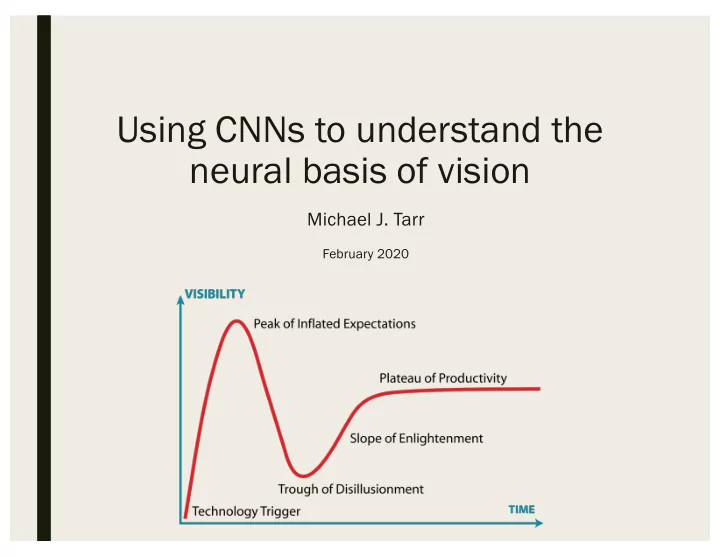
Using CNNs to understand the neural basis of vision Michael J. Tarr - - PowerPoint PPT Presentation

Using CNNs to understand the neural basis of vision

Michael J. Tarr

February 2020

AI Space

Cognitive Plausibility Biological Plausibility Performance Humans Early AI 1980’s- 2000’s PDP “Deep” AI Future?

Different kinds of AI (in practice)

1. AI that maximizes performance – e.g., diagnosing disease – learns and applies knowledge humans might not typically learn/apply – “who cares if it does it like humans or not” 2. AI that is meant to simulate (to better understand) cognitive or biological processes – e.g., PDP – specifically constructed so as to reveal aspects of how biological systems learn/reason/etc. – understanding at the neural or cognitive levels (or both) 3. AI that performs well and helps understand cognitive or biological processes – e.g., Deep learning models (cf. Yamins/DiCarlo) – “representational learning” 4. AI that is specifically designed to predict human performance/preference – e.g., Google/Netflix/etc. – only useful if it predicts what humans actually do or want

A Bit More on Deep Learning

• Typically relies on supervised learning – 1,000,000’s of labeled inputs
• Labels are a metric of human performance – so long as the network learns the

correct input->label mapping, it will perform “well” by this metric

• However, the network can’t do better than the labels
• Features might exist in the input that would improve performance, but

unless those features are sometimes correctly labeled, the model won’t learn that feature to output mapping

• The network can reduce misses, but it can’t discover new mappings unless there

are existing further correlations between input->labels in the trained data

• So Deep Neural Networks tend to be very good at the kinds of AI that predicts

human performance (#4) and that maximize performance (#1), but the jury is still out on AI that performs well and helps us understand biological intelligence (#3); might also be used for simulation of biological intelligence (#2)

Some Numbers (ack)

• Retinal input (~108 photoreceptors) undergoes a 100:1 data

compression, so that only 106 samples are transmitted by the optic nerve to the LGN

• From LGN to V1, there is almost a 400:1 data expansion, followed

by some data compression from V1 to V4

• From this point onwards, along the ventral cortical stream, the

number of samples increases once again, with at least ~109 neurons in so-called “higher-level” visual areas

• Neurophysiology of V1->V4 suggests a feature hierarchy, but even

V1 is subject to the influence of feedback circuits – there are ~2x feedback connections as feedforward connections in human visual cortex

• Entire human brain is about ~1011 neurons with ~1015 synapses

The problem

Ways of collecting brain data

■ Br Brai ain Par arts List - Define all the types of neurons in the brain ■ Co Connect ctome - Determine the connection matrix of the brain ■ Br Brai ain Activity Map ap - Record the activity of all neurons at msec precision (“functional”)

– Record from individual neurons – Record aggregate responses from 1,000,000’s of neurons

■ Be Behavior Prediction/Ana nalys ysis - Build predictive models of complex networks or complex behavior ■ Potential Connections to a variety of other data sources, including genomics, proteomics, behavioral economics

Neuroimaging Challenges

■ Ex Expen ensive ■ La Lack of power er – both in number of observations (1000’s at best) and number of individuals (100’s at best) ■ Va Variation – aligning structural or functional brain maps across different individuals ■ An Analysi ysis – high-dimensional data sets with unknown structure ■ Tr Tradeoffs between spatial and temporal resolution and invasiveness

Tradeoffs in neuroimaging

WANT TO BE HERE WE ARE HERE

Background

■ There is a long-standing, underlying assumption that vision is compositional – “High-level” representations (e.g., objects) are comprised of separable parts (“building blocks”) – Parts can be recombined to represent different things – Parts are the consequence of a progressive hierarchy of increasing complex features comprised of combinations of simpler features ■ Visual neuroscience has often focused on the nature of such features – Both intermediate (e.g., V4) and higher-level (e.g., IT) – Toilet brushes – Image reduction – Genetic algorithms

Tanaka (2003) used an image reduction method to isolate “critical features” (physiology)

Woloszyn and Sheinberg (2012)

Firing Rate (Hz)

50 100 150

Firing Rate (Hz)

50 100 150

Firing Rate (Hz)

50 100

Firing Rate (Hz)

50 100

A C D

Rank 1 Rank 2 Rank 3

Firing Rate (Hz)

B E F

Firing Rate (Hz)

50 100 Rank 4 Rank 5

Frustrating Progress

■ Few, if any, studies have made much progress in illuminating the building blocks of vision – Some progress at the level of V4? – Almost no progress at the level of IT – Typical account of neural selectivity is in terms of:

■ Reified categories – face patches – functional selectivity of neurons

• r neural regions is defined in terms of the category for which it

seems most preferential – Ignores the relatively gentle similarity gradient – Ignores the failure to conduct an adequate search of the space ■ Features that do not seem to support generalization/composition – Fail on ocular inspection and any computational predictions – Again ignores the failure to conduct an adequate search of the space

What to do?

■ Collect much more data – across millions of different images and millions of neurons ■ Better search algorithms based on real-time feedback ■ Run simulations of a vision system – Align task(s) with biological vision systems – Align architecture with biological vision systems – Must be high performing (or what is the point?) – Explore the functional features that emerge from the simulation ■ Not much progress on this front until recently…CNNs/Deep Networks

Stupid CNN Tricks

• Hierarchical correspondence
• Visualization of “neurons”

[Digression – is visualization a good metric for evaluating models?]

HCNNs are good candidates for models of the ventral visual pathway

Yamins & DiCarlo

Goal-Driven Networks as Neural Models

• whatever parameters are used, a neural network will have to be

effective at solving the behavioral tasks the sensory system supports to be a correct model of a given sensory system

• so… advances in computer vision, etc. that have led to high-

performing systems – that solve behavioral tasks nearly as effectively as we do – could be correct models of neural mechanisms

• conversely, models that are ineffective at a given task are

unlikely to ever do a good job at characterizing neural mechanisms

Approach

• Optimize network parameters for performance on a reasonable,

ecologically—valid task

• Fix network parameters and compare the network to neural

data

• Easier than “pure neural fitting” b/c collecting millions of

human-labeled images is easier than obtaining comparable neural data

Key Questions

• Do such top-down goals – tasks – constrain biological

structure?

• Will performance optimization be sufficient to cause

intermediate units in the network to behave like neurons?

“Neural-like” models via performance optimization

layer 2 layer 3 layer 4

. . .

Behavioral Tasks

e.g. Trees vs non-Trees

• 1. Optimize Model for Task Performance

Neural Recordings from IT and V4

layer 1

⊗ ⊗ ⊗ Filter Threshold Pool Normalize Operations in Linear-Nonlinear Layer

Performance Low Variation Tasks High Variation Tasks

Pixels SIFT V1-like V2-like HMAX PLOS09 HMO V4 Population IT Population Humans Medium Variation Tasks

100ms Visual Presentation

. . .

V1 IT V2 V4

• 2. Test Per-Site Neural Predictions

High-variation V4-to-IT Gap

100 80 60 40 20 LN LN

LN LN . . . LN LN LN . . . LN

LN LN . . . . . . . . . Spatial Convolution

• ver Image Input

A B

Yamins et al.

Model Performance/IT- Predictivity Correlation

IT Explained Variance (%) 0.6 0.7 0.5

Categorization Performance Optimization (r =0.78) IT Fitting Optimization (r =0.80) Random Selection (r =0.55)

Categorization Performance (balanced accuracy) 30 15 –15

B

V2-like HMAX PLOS09 SIFT r = 0.87 ± 0.15 Category Ideal Observer

0.6 0.8 1.0

HMO

50 40 30 20 10

V1-like Pixels

A

Yamins et al.

IT Neural Predictions

HMO Layer 1 (4%) Category Ideal Observer (15%) HMO Layer 2 (21%) HMO Layer 3 (36%) HMO Top Layer (48%) V2-Like Model (26%) HMAX Model (25%) V1-Like Model (16%) IT Site 150 IT Site 56 IT Site 42

Response Magnifude

HMO Layers Control Models

Animals Planes Boats Cars Chairs Faces Fruits Tables

(n=168)

Binned Site Counts

IT Explained Variance (%)

Ideal Observers Control Models HMO Layers Category All Variables Pixels V1-Like PLOS09 HMAX V2-Like HMO L1 HMO L2 HMO L3 HMO Top SIFT

A B

Single Site Explained Variance (%)

C

Yamins et al.

Human fMRI

d

HCNN model Human IT (fMRI)

Animate Human Not human Body Face Body Face Natural Artificial Inanimate

A = 0.38 ** **** **** **** **** ****

e

0.2 0.4 0.2 0.4 Human V1–V3 Human IT RDM voxel correlation (Kendall’s A) Scores Layer 1 Layer 2 Layer 3 Layer 4 Layer 5 Layer 6 Layer 7 Layer 1 Layer 2 Layer 3 Layer 4 Layer 5 Layer 6 Layer 7 Convolutional Fully connected

**** **** **** * **** **** **** ****

SVM Geometry- supervised

****

Figure 2 Goal-driven optimization yields neurally predictive models of ventral visual cortex. (a) HCNN models that are better optimized to solve

• Khaligh-Razavi & Kriegeskorte

Do deep networks and humans perform this sort of task in the same way?

Two important differences:

• 1. People learn from fewer examples
• 2. People learn “richer” representations

§ Decomposable into parts § Learn a concept that can be flexibly applied

• Generate new examples
• Parse an object into parts and their relations
• Generalize to new instances of the overall class

• Duh. The particular model being tested did not have

general world knowledge/context – it only was intended to perform captioning using simple object and scene labeling (~semantics)

Ponce et al.

A) Used pre-trained deep generative network (Dosovitskiy and Brox, 2016) B) Random textures C) Animals fixated while images were presented D) Neuronal responses were used to select top 10 images from prior generation plus 30 new, generated codes 250 generations

Evolution of preferred units for the network

■ Validation of the method within the artificial neural network – Models of biological neurons? ■ “Super Stimuli” for units within the network – Most evolved images activated artificial units more strongly than all of 1.4+ million images in ImageNet ■ Network can recover the preferred stimuli of units constructed to have a single preferred image

Layer 1 fc8 four layers, 100 random units

Evolution of preferred stimuli by one biological neuron (PIT)

(A) Mean response to synthetic (black) and reference (green) images for every generation (spikes per s ± SEM). (B) Last-generation images evolved during three independent evolution experiments; the leftmost image corresponds to the evolution in (A); the other two evolutions were carried out on the same single unit on different days. Left half of each image is the contralateral visual field for this recording site. Average of the top 5 images from the final generation. (C) The top 10 images from this image set for this neuron. (D) The worst 10 images from this image set for this neuron. (E) The selectivity of this neuron to different image categories (2,550 natural images plus selected synthetic images). Early = best image from each of the first 10 generations; Late = last 10. Average over 10–12 repeated presentations.

Evolution of preferred stimuli in other neurons

46 evolution experiments on single- and multi-unit sites in IT on six different monkeys Synthetic images consistently evolved to become increasingly effective stimuli; firing rate change (A) Neurons’ maximum responses to natural versus evolved images were significantly different (B) Histogram of response magnitudes for PIT cell Ri-10 to the top synthetic image in each

• f the 210 generations and responses to

each of the 2,550 natural images (C) (D) One of the instances where natural images evoked stronger responses than did synthetic images

Evolution of preferred stimuli in other neurons

Each pair of images shows the last-generation synthetic images from two independent experiments for a single recording site. To the right are the top 10 images for each neuron from a natural image set.

Neural population control via deep image synthesis Bashivan, Kar, & DiCarlo (2019)

Responses

Cat

C D

The neural control experiments are done in four steps. (1) Parameters of the neural network are optimized by training on a large set of labeled natural images (Imagenet) and then held constant thereafter. (2) ANN “neurons” are mapped to each recorded V4 neural site. The mapping function constitutes an image-computable predictive model of the activity of each of those V4 sites. (3) The resulting differentiable model is then used to synthesize “controller” images for either single-site or population control. (4) The luminous power patterns specified by these images are then applied by the experimenter to the subject’s retinae and the degree of control of the neural sites is measured.

Why should computer scientists and brain scientists talk?

■ Th Theo eory – how do we understand the principles of computation in biological systems? ■ Imp Implementa tati tion – how do we build intelligent machines? ■ Si Simulation – how do we understand emergent phenomena in complex systems? ■ Da Data – how do we uncover regularities in large-scale data?

Humans are falliable

Cautionary quotes

■ To substitute an ill-understood model of the world for the ill- understood world is not progress. — P. J. Richerson and R. Boyd in The Latest on the Best, Dupré (ed.) ■ Tarr’s coda on this: To substitute a bad model of the world for the ill-understood world is also not progress.