Update on the Color Transparency Experiment e' p 16 July 2020 e - - PowerPoint PPT Presentation

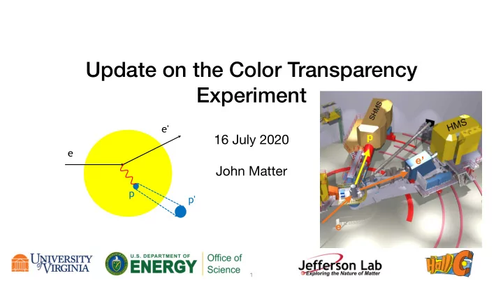
16 July 2020 John Matter

1

e e' p p'

Update on the Color Transparency Experiment

e e’ p

Summary

• CT definition
• Optics
• Target Boiling
• Proton Absorption
• PID efficiency
• Livetime
• Tracking
• Luminosity Scan (carbon "boiling")
• Systematic Uncertainty
• Results

2

e e' p p'

CT onset 1.0 Q02 Q2➝

Complete transparency Glauber

Color Transparency

3

• Color Transparency
• Vanishing of final/initial state interactions in

exclusive processes at large momentum transfer

• Squeezing
• Scattering of point-like configurations
• Small transverse size ⇒ attenuated strong

interaction; color-neutral singlet

• Freezing
• Small size maintained as the hadron

passes through nucleus

A(𝝆,di-jet): FNAL A(𝛅, 𝝆- p): Jlab A(e, e’𝝆+): JLab A(e, e’𝛓0): DESY & JLab

u ū

Meson CT Experiments

A(p,2p): BNL A(e,e’p): SLAC, JLab

u u d

Baryon

Color Transparency

4

CT onset 1.0 Q02 Q2➝

Complete transparency Glauber

• Define transparency T as the ratio
• f the cross section for a given

process on a bound nucleon to the cross section for the same process on a free nucleon

• Glauber predicts constant T
• CT predicts a rise in T
• CT onset observed in meson

production; baryon results are ambiguous.

• Where is the onset?

No onset… yet?

Previous Measurements A(e,e’p)

5

PRL 72, 1986 (1994) PRB 351, 87 (1995) PRL 80, 5072 (1998) PRC 66, 044613 (2002) PRC 72, 054602 (2005) PRC 45, 780 (1992)

Solid points = JLab Open points = other

E12-06-107

6

• First 12 GeV era Hall C

experiment in early 2018

• Coincidence trigger
• SHMS = proton
• HMS = electron
• Targets
• 10 cm LH2 (Hee’p check)
• 6% 12C (production)
• Al dummy (LH2 background)

e e’ p

E12-06-107

7

Q2 [GeV2] SHMS angle [deg] SHMS central P [GeV/c] HMS angle [deg] HMS central P [GeV/c] 8.0 17.1 5.122 45.1 2.131 9.5 21.6 5.925 23.2 5.539 11.5 17.8 7.001 28.5 4.478 14.3 12.8 8.505 39.3 2.982 6 . 4 G e V b e a m 10.6 GeV beam

• E12-06-107

12C(e,e’p)

8

Optics (Holly Szumila-Vance)

Blue = data Green = MC w/o radiative effects Red = MC w/ radiative effects

W

Emiss [Gev]

C12, Q2=8 GeV2

Emiss Pmiss

0.3 − 0.2 − 0.1 − 0.1 0.2 0.3 20 40 60 80 100 120 140 160

Pmiss [Gev]

C12, Q2=8 GeV2

9

LH2 data

Missing momentum is one of

• ur most sensitive parameters,

as it depends on momentum and angle in both spectrometers

Optics (Holly Szumila-Vance & Deepak Bhetuwal)

y = m ∗ Ibeam + b ⇒ y b = m b ∗ Ibeam + 1

Divide by the offset parameter
 to re-normalize data to unity

Fit slope represents ‘fractional yield loss per uA’

10

Target boiling (Carlos Yero)

y

https://hallcweb.jlab.org/DocDB/0010/001023/001/April2018_BoilingStudies.pdf

11

SHMS Proton Absorption

y

• Based on the materials in the proton’s path, I

estimate absorption to be 8.9%*

• From CT data, I estimate 8.5 ± 0.5%
• 1. Place tight SHMS acceptance cuts on good ep

coincidences

• 2. Pick tight HMS-only cuts that produce the same

distributions

• 3. Calculate yields from ep coincidence and HMS

singles data

• For comparison, Carlos estimates 4.66 ± 0.47% in

the HMS

• https://hallcweb.jlab.org/DocDB/

0010/001020/002/ProtonAbsorption_slides.pdf

A = 1 − exp {−∑ xi λi} A = 1 − Ycoin Ysingles

* https://docs.google.com/spreadsheets/d/1LeaFrQjKTuOeliKTEN8QAHqDkFCYzW18bMMjTKu1ejQ

12

PID Efficiency
 Calculated per delta bin, then weighted

y

6 − 4 − 2 − 2 4 6 8 0.9 0.92 0.94 0.96 0.98 1

δ

ϵi

¯ ϵ = ∑i wiϵi ∑j wj

ϵi = ni,did ni,should

wi = 1/σ2

i

HMS SHMS Calorimeter Cherenkov 8 9.5 11.5 14.3 8 9.5 11.5 14.3 0.96 0.97 0.98 0.99 1.00 0.96 0.97 0.98 0.99 1.00

Q2 [GeV2] efficiency target

C12_thick LH2

13

Livetime

y

• Place appropriate BCM cuts
• T = number of accepted triggers

(T.shms.pTRIG1_tdcTimeRaw!=0)

• S = scaler counts

(P .pTRIG1.scaler)

• Prescale factor P=1+2^(ps-1)
• CLTA = P * T / S

99.8 99.9 100.0 0.003 0.004 0.005 0.006

pTRIG6 Rate [kHz] CLTA as.factor(Q2)

8 9.5 11.5 14.3

target

C12_thick C12_thin LH2

SHMS CLTA = TpTRIG6/SpTRIG6

92 93 94 95 96 97 98 99 100 101 102 25 50 75 100

pTRIG1 Rate [kHz] LTE as.factor(Q2)

8 9.5 11.5 14.3

target

C12_thick C12_thin LH2

SHMS LTE = TEDTM/SEDTM

14

Livetime

y

• Place appropriate BCM cuts
• T = number of accepted triggers

(T.coin.pEDTM_tdcTimeRaw!=0)

• S = scaler counts

(P .pEDTM.scaler)

• LTE = T / S

HMS SHMS Tracking 8 9.5 11.5 14.3 8 9.5 11.5 14.3 0.97 0.98 0.99 1.00

Q2 [GeV2] efficiency target

C12_thick LH2

15

Tracking Efficiency

y

• Select events that should form a track

(PID cut) && P.hod.betanotrack < 1.2


&& (fewer than 21 hits per DC)
 && P.hod.goodscinhit==1
 && P.hod.goodstarttime==1

• How many did?

P.dc.ntrack==1 ||


(P.dc.ntrack>1 && abs(P.gtr.dp)<15
 && abs(P.gtr.y)<5
 && abs(P.gtr.th)<0.2
 && abs(P.gtr.ph)<0.2
 && -10 < P.hod.1x.fptime < 5
 && P.hod.1x.totNumGoodNegAdcHits<5
 && (same two cuts for 1y, 2x, 2y))

16

Luminosity Scan 1

y

• 180

182 184 20 40 60

BCM4A Current [uA] Charge normalized yield [#/uC]

Corrected Yield

• SHMS runs 1992–2000, each with different

steady currents between 2 uA and 65 uA

• C12 0.5% target
• Calculate yields and correct for detector

efficiency, livetime, and prescale factor

• Calculating precent change in yield per uA, we

get 0.008 ± 0.010% which is consistent with zero

• Typical currents for CT data are 50 uA, or

0.4% per uA

b = 181.79 ± 0.74 Y = m * I + b m = 0.014 ± 0.019

17

Luminosity Scan 2

y

• SHMS runs 3109–3114, each with different

steady currents between 2.5 uA and 60 uA

• C12 1.5% target
• Calculate yields and correct for detector

efficiency, livetime, and prescale factor

• I’m still working on this, but Deepak’s result is
• 0.1%/uA
• Can estimate systematic uncertainty for livetime,

PID, and tracking from the difference between the results of these two luminosity scans

• Based on Deepak’s results, we expect 0.5%

systematic uncertainty due to livetime and efficiency corrections

in progress

E12-06-107

18

TABLE II. Systematic Uncertainties Source Q2 dependent uncertainty (%) Spectrometer acceptance 3.0 Event selection 1.5 Tracking efficiency Radiative corrections 1.0 Live time correction Source Normalization uncertainty (%) Free cross section 2.0 Target thickness 0.5 Beam charge 1.0 Proton absorption 0.5 Total

12

1 2 3

• 1. Preliminary number based on agreement between Pm

spectra from simc and data

• 2. See cut study at https://hallcweb.jlab.org/elogs/

Color+Transparency/48

• 3. Determined from variation in corrections for different model

parameter choices

0.995+/-0.008

19

E12-06-107 Final H(e,e’p) results

• Ratio of yields from data to simc should be 1
• Ingredients:
• Livetime
• Tracking, hodo, PID efficiency
• Target boiling
• Em, Pm < 50 MeV
• simc form factor is Peter’s fit* from 1995

*P

. E. Bosted, Phys. Rev. C 51, 409 (1995)

• Preliminary results consistent with no increase in

transparency

• H(e,e’p) analysis finished
• Final C12 transparency soon
• Still need:
• Final luminosity scan (to determine

systematic uncertainty from efficiency and livetime corrections)

• Convergence of my work and Deepak’s
• A publication of these CT results will be

ready to circulate once we complete these cross checks

20

E12-06-107 C12 transparency

21

This work was supported by the DOE Office of Science
 (U.S. DOE Grant Number: DE-FG02-07ER41528)

Thank you!