Uniform Convergence - Sample Complexity Assume that we want to - - PowerPoint PPT Presentation

Uniform Convergence - Sample Complexity

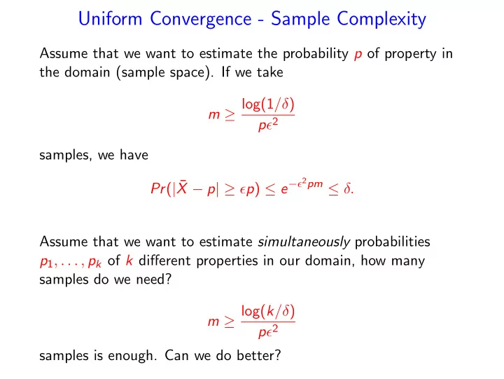
Assume that we want to estimate the probability p of property in the domain (sample space). If we take m ≥ log(1/δ) pǫ2 samples, we have Pr(| ¯ X − p| ≥ ǫp) ≤ e−ǫ2pm ≤ δ. Assume that we want to estimate simultaneously probabilities p1, . . . , pk of k different properties in our domain, how many samples do we need? m ≥ log(k/δ) pǫ2 samples is enough. Can we do better?

What’s Learning?

Two types of learning: What’s a rectangle?

• ”A rectangle is any quadrilateral with four right angles”
• Here are many random examples of rectangles, here are many

random examples of shapes that are not rectangles. Make your own rule that best conforms with the examples - Statistical Learning.

Statistical Learning – Learning From Examples

• We want to estimate the working temperature range of an

iPhone.

– We could study the physics and chemistry that affect the performance of the phone – too hard – We could sample temperatures in [-100C,+100C] and check if the iPhone works in each of these temperatures – We could sample users’ iPhones for failures/temperature

• How many samples do we need?
• How good is the result?
• 100C

+100C a b

Learning From Examples

• We get n random training examples from distribution D. We

choose a rule [a, b] conforms with the examples.

• We use this rule to decide on the next example.
• If the next example is drawn from D, what is the probability

that we is wrong?

• Let [c, d] be the correct rule.
• Let ∆ = ([a, b] − [c, d]) ∪ ([c, d] − [a, b])
• We are wrong only on examples in ∆.

What’s the probability that we are wrong?

• We are wrong only on examples in ∆.
• The probability that we are wrong is the probability of having

a quary from ∆.

• If Prob(sample from ∆) ≤ ǫ we don’t care.
• If Prob(sample from ∆) ≥ ǫ then the probability that n

training samples all missed ∆, is bounded by (1 − ǫ)n = δ, for n ≥ 1

ǫ log 1 δ.

• Thus, with n ≥ 1

ǫ log 1 δ training samples, with probability

1 − δ, we chose a rule (interval) that gives the correct answer for quarries from D with probability ≥ 1 − ǫ.

Learning a Binary Classifier

• An unknown probability distribution D on a domain U
• An unknown correct classification – a partition c of U to In

and Out sets

• Input:
• Concept class C – a collection of possible classification rules

(partitions of U).

• A training set {(xi, c(xi)) | i = 1, . . . , m}, where x1, . . . , xm are

sampled from D.

• Goal: With probability 1 − δ the algorithm generates a good

classifier. A classifier is good if the probability that it errs on an item generated from D is ≤ opt(C) + ǫ, where opt(C) is the error probability of the best classifier in C.

Learning a Binary Classifier

• Out and In items, and a concept class C of

possible classifica;on rules

When does the sample identify the correct rule? - The realizable case

• The realizable case - the correct classification c ∈ C.
• For any h ∈ C let ∆(c, h) be the set of items on which the

two classifiers differ: ∆(c, h) = {x ∈ U | h(x) = c(x)}

• Algorithm: choose h∗ ∈ C that agrees with all the training set

(there must be at least one).

• If the sample (training set) intersects every set in

{∆(c, h) | Pr(∆(c, h)) ≥ ǫ}, then Pr(∆(c, h∗)) ≤ ǫ.

Learning a Binary Classifier

• Red and blue items, possible classifica9on

rules, and the sample items

When does the sample identify the correct rule? The unrealizable (agnostic) case

• The unrealizable case - c may not be in C.
• For any h ∈ C, let ∆(c, h) be the set of items on which the

two classifiers differ: ∆(c, h) = {x ∈ U | h(x) = c(x)}

• For the training set {(xi, c(xi)) | i = 1, . . . , m}, let

˜ Pr(∆(c, h)) = 1 m

m

• i=1

1h(xi)=c(xi)

• Algorithm: choose h∗ = arg minh∈C ˜

Pr(∆(c, h)).

• If for every set ∆(c, h),

|Pr(∆(c, h)) − ˜ Pr(∆(c, h))| ≤ ǫ, then Pr(∆(c, h∗)) ≤ opt(C) + 2ǫ. where opt(C) is the error probability of the best classifier in C.

If for every set ∆(c, h), |Pr(∆(c, h)) − ˜ Pr(∆(c, h))| ≤ ǫ, then Pr(∆(c, h∗)) ≤ opt(C) + 2ǫ. where opt(C) is the error probability of the best classifier in C. Let ¯ h be the best classifier in C. Since the algorithm chose h∗, ˜ Pr(∆(c, h∗)) ≤ ˜ Pr(∆(c, ¯ h)). Thus, Pr(∆(c, h∗)) − opt(C) ≤ ˜ Pr(∆(c, h∗)) − opt(C) + ǫ ≤ ˜ Pr(∆(c, ¯ h)) − opt(C) + ǫ ≤ 2ǫ

Detection vs. Estimation

• Input:
• Concept class C – a collection of possible classification rules

(partitions of U).

• A training set {(xi, c(xi)) | i = 1, . . . , m}, where x1, . . . , xm are

sampled from D.

• For any h ∈ C, let ∆(c, h) be the set of items on which the

two classifiers differ: ∆(c, h) = {x ∈ U | h(x) = c(x)}

• For the realizable case we need a training set (sample) that

with probability 1 − δ intersects every set in {∆(c, h) | Pr(∆(c, h)) ≥ ǫ} (ǫ-net)

• For the unrealizable case we need a training set that with

probability 1 − δ estimates, within additive error ǫ, every set in ∆(c, h) = {x ∈ U | h(x) = c(x)} (ǫ-sample).

Uniform Convergence Sets

Given a collection R of sets in a universe X, under what conditions a finite sample N from an arbitrary distribution D over X, satisfies with probability 1 − δ,

1

∀r ∈ R, Pr

D (r) ≥ ǫ ⇒ r ∩ N = ∅

(ǫ-net)

2 for any r ∈ R,

• Pr

D (r) − |N ∩ r|

|N|

• ≤ ε

(ǫ-sample)

Learnability - Uniform Convergence

Theorem In the realizable case, any concept class C can be learned with m = 1

ǫ(ln |C| + ln 1 δ) samples.

Proof. We need a sample that intersects every set in the family of sets {∆(c, c′) | Pr(∆(c, c′)) ≥ ǫ}. There are at most |C| such sets, and the probability that a sample is chosen inside a set is ≥ ǫ. The probability that m random samples did not intersect with at least one of the sets is bounded by |C|(1 − ǫ)m ≤ |C|e−ǫm ≤ |C|e−(ln |C|+ln 1

δ ) ≤ δ.

How ¡Good ¡is ¡this ¡Bound? ¡

• Assume ¡that ¡we ¡want ¡to ¡es3mate ¡the ¡working ¡

temperature ¡range ¡of ¡an ¡iPhone. ¡

• We ¡sample ¡temperatures ¡in ¡[-­‑100C,+100C] ¡

and ¡check ¡if ¡the ¡iPhone ¡works ¡in ¡each ¡of ¡these ¡

• temperatures. ¡
• ­‑100C ¡

+100C ¡ a ¡ b ¡

Learning an Interval

• A distribution D is defined on universe that is an interval

[A, B].

• The true classification rule is defined by a sub-interval

[a, b] ⊆ [A, B].

• The concept class C is the collection of all intervals,

C = {[c, d] | [c, d] ⊆ [A, B]} Theorem There is a learning algorithm that given a sample from D of size m = 2

ǫ ln 2 δ, with probability 1 − δ, returns a classification rule

(interval) [x, y] that is correct with probability 1 − ǫ. Note that the sample size is independent of the size of the concept class |C|, which is infinite.

Learning ¡an ¡Interval ¡

• If ¡the ¡classifica2on ¡error ¡is ¡≥ ¡ε ¡then ¡the ¡sample ¡

missed ¡at ¡least ¡one ¡of ¡the ¡the ¡intervals ¡[a,a’] ¡

• r ¡[b’,b] ¡each ¡of ¡probability ¡≥ ¡ε/2 ¡

A ¡ B ¡ a ¡ b ¡ x ¡ y ¡ ε/2 ¡ a’ ¡

Each ¡sample ¡excludes ¡many ¡possible ¡intervals. ¡ The ¡union ¡bound ¡sums ¡over ¡overlapping ¡hypothesis. ¡ Need ¡beIer ¡characteriza2on ¡of ¡concept's ¡complexity! ¡ ¡

ε/2 ¡ ¡ b’ ¡

Proof. Algorithm: Choose the smallest interval [x, y] that includes all the ”In” sample points.

• Clearly a ≤ x < y ≤ b, and the algorithm can only err in

classifying ”In” points as ”Out” points.

• Fix a < a′ and b′ < b such that Pr([a, a′]) = ǫ/2 and

Pr([b, b′]) = ǫ/2.

• If the probability of error when using the classification [x, y] is

≥ ǫ then either a′ ≤ x or y ≤ b′ or both.

• The probability that the sample of size m = 2

ǫ ln 2 δ did not

intersect with one of these intervals is bounded by 2(1 − ǫ 2)m ≤ e− ǫm

2 +ln 2 ≤ δ

• The union bound is far too loose for our applications. It sums
• ver overlapping hypothesis.
• Each sample excludes many possible intervals.
• Need better characterization of concept’s complexity!

Probably Approximately Correct Learning (PAC Learning)

• The goal is to learn a concept (hypothesis) from a pre-defined

concept class. (An interval, a rectangle, a k-CNF boolean formula, etc.)

• There is an unknown distribution D on input instances.
• Correctness of the algorithm is measured with respect to the

distribution D.

• The goal: a polynomial time (and number of samples)

algorithm that with probability 1 − δ computes an hypothesis

• f the target concept that is correct (on each instance) with

probability 1 − ǫ.

Formal Definition

• We have a unit cost function Oracle(c, D) that produces a

pair (x, c(x)), where x is distributed according to D, and c(x) is the value of the concept c at x. Successive calls are independent.

• A concept class C over input set X is PAC learnable if there is

an algorithm L with the following properties: For every concept c ∈ C, every distribution D on X, and every 0 ≤ ǫ, δ ≤ 1/2,

• Given a function Oracle(c, D), ǫ and δ, with probability 1 − δ

the algorithm output an hypothesis h ∈ C such that PrD(h(x) = c(x)) ≤ ǫ.

• The concept class C is efficiently PAC learnable if the algorithm

runs in time polynomial in the size of the problem,1/ǫ and 1/δ.

———— So far we showed that the concept class ”intervals on the line” is efficiently PAC learnable.

Learning Axis-Aligned Rectangle

• Concept class: all axis aligned rectangles.
• Given m samples {xi, yi, class}, i = 1, . . . , m.
• Let R′ be the smallest rectangle that contains all the positive
• examples. A(R′) the corresponding algorithm.
• Let R be the correct concept. W.l.o.g. Pr(R) > ǫ
• Define 4 sides each with probability ǫ/4 of R: r1, r2, r3, r4.
• If Pr(A(R′)) ≥ ǫ) then there is an i ∈ {1, 2, 3, 4} such that

Pr(R′ ∩ ri) ≥ ǫ/4, and there were no training examples in R′ ∩ ri Pr(A(R′)) ≥ ǫ) ≤ 4(1 − ǫ/4)m

Learning Axis-Aligned Rectangle - More than One Solution

• Concept class: all axis aligned rectangles.
• Given m samples {xi, yi, class}, i = 1, . . . , m.
• Let R′ be the smallest rectangle that contains all the positive

examples.

• Let R′′ be the largest rectangle that contain no negative

examples.

• Let R be the correct concept.

R′ ⊆ R ⊆ R′′

• Define 4 sides (in for R′, out for R′′) each with probability 1/4
• f R: r1, r2, r3, r4.

Pr(A(R′)) ≥ ǫ) ≤ 4(1 − ǫ/4)m

Learning Boolean Conjunctions

• A Boolean literal is either x or ¯

x.

• A conjunction is xi ∧ xj ∧ ¯

xk....

• C = is the set of conjunctions of up to 2n literals.
• The input space is {0, 1}n

Theorem The class of conjunctions of Boolean literals is efficiently PAC learnable.

Proof

• Start with the hypothesis h = x1 ∧ ¯

x1 ∧ . . . xn ∧ ¯ xn.

• Ignore negative examples generated by Oracle(c, D).
• For a positive example (a1, . . . , an), if ai = 1 remove ¯

xi,

• therwise remove xi from h.

Lemma At any step of the algorithm the current hypothesis never errs on negative example. It may err on positive examples by not removing enough literals from h. Proof. Initially the hypothesis has no satisfying assignment. It has a satisfying assignment only when no literal and its complement are left in the hypothesis. A literal is removed when it contradicts a positive example and thus cannot be in c. Literals of c are never

• removed. A negative example must contradict a literal in c, thus is

not satisfied by h.

Analysis

• The learned hypothesis h can only err by rejecting a positive
• examples. (it rejects a input unless it had a similar positive

example in the training set.)

• If h errs on a positive example then in has a literal that is not

in c.

• Let z be a literal in h and not c. Let

p(z) = Pra∼D(c(a) = 1 and z = 0 in a).

• A literal z is“bad” If p(z) >

ǫ 2n.

• Let m ≥ 2n

ǫ ln(2n) + ln 1 δ. The probability that after m samples

there is any bad literal in the hypothesis is bounded by 2n(1 − ǫ 2n)m ≤ δ.

Two fundamental questions:

• What concept classes are PAC-learnable with a given number
• f training (random) examples?
• What concept class are efficiently learnable (in polynomial

time)? A complete (and beautiful) characterization for the first question, not very satisfying answer for the second one. Some Examples:

• Efficiently PAC learnable: Interval in R, rectangular in R2,

disjunction of up to n variables, 3-CNF formula,...

• PAC learnable, but not in polynomial time (unless P = NP):

DNF formula, finite automata, ...

• Not PAC learnable: Convex body in R2,

{sin(hx) | 0 ≤ h ≤ π} ,...

Uniform Convergence [Vapnik – Chervonenkis 1971]

Definition A set of functions F has the uniform convergence property with respect to a domain Z if there is a function mF(ǫ, δ) such that

• for any ǫ, δ > 0, m(ǫ, δ) < ∞
• for any distribution D on Z, and a sample z1, . . . , zm of size

m = mF(ǫ, δ), Pr(sup

f ∈F

| 1 m

m

• i=1

f (zi) − ED[f ]| ≤ ǫ) ≥ 1 − δ. Let fE(z) = 1z∈E then E[fE(z)] = Pr(E).

Uniform Convergence and Learning

Definition A set of functions F has the uniform convergence property with respect to a domain Z if there is a function mF(ǫ, δ) such that

• for any ǫ, δ > 0, m(ǫ, δ) < ∞
• for any distribution D on Z, and a sample z1, . . . , zm of size

m = mF(ǫ, δ), Pr(sup

f ∈F

| 1 m

m

• i=1

f (zi) − ED[f ]| ≤ ǫ) ≥ 1 − δ.

• Let FH = {fh | h ∈ H}, where fh is the loss function for

hypothesis h.

• FH has the uniform convergence property ⇒ an ERM

(Empirical Risk Minimization) algorithm ”learns” H.

• The sample complexity of learning H is bounded by mFH(ǫ, δ)

Uniform Convergence - 1971, PAC Learning - 1984

Definition A set of functions F has the uniform convergence property with respect to a domain Z if there is a function mF(ǫ, δ) such that

• for any ǫ, δ > 0, m(ǫ, δ) < ∞
• for any distribution D on Z, and a sample z1, . . . , zm of size

m = mF(ǫ, δ), Pr(sup

f ∈F

| 1 m

m

• i=1

f (zi) − ED[f ]| ≤ ǫ) ≥ 1 − δ.

• Let FH = {fh | h ∈ H}, where fh is the loss function for

hypothesis h.

• FH has the uniform convergence property ⇒ an ERM

(Empirical Risk Minimization) algorithm ”learns” H. PAC efficiently learnable if there a polynomial time ǫ, δ-approximation for minimum ERM.

• The sample complexity of learning H is bounded by m

(ǫ, δ)

Uniform Convergence

Definition A set of functions F has the uniform convergence property with respect to a domain Z if there is a function mF(ǫ, δ) such that

• for any ǫ, δ > 0, m(ǫ, δ) < ∞
• for any distribution D on Z, and a sample z1, . . . , zm of size

m = mF(ǫ, δ), Pr(sup

f ∈F

| 1 m

m

• i=1

f (zi) − ED[f ]| ≤ ǫ) ≥ 1 − δ. VC-dimension and Rademacher complexity are the two major techniques to

• prove that a set of functions F has the uniform convergence

property

• charaterize the function mF(ǫ, δ)

Some Background

• Let fx(z) = 1z≤x (indicator function of the event {−∞, x})
• Fm(x) = 1

m

m

i=1 fx(zi) (empirical distributed function)

• Strong Law of Large Numbers: for a given x,

Fm(x) →a.s F(x) = Pr(z ≤ x).

• Glivenko-Cantelli Theorem:

sup

x∈R

|Fm(x) − F(x)| →a.s 0.

• Dvoretzky-Keifer-Wolfowitz Inequality

Pr(sup

x∈R

|Fm(x) − F(x)| ≥ ǫ) ≤ 2e−2nǫ2.

• VC-dimension characterizes the uniform convergence property

for arbitrary sets of events.