UMBC A B M A L T F O U M B C I M Y O R T 1 - - PowerPoint PPT Presentation

Digital Systems Transmission Lines VI CMPE 650 1 (4/3/08)

UMBC

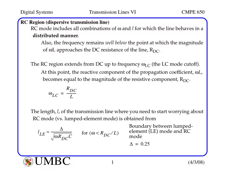
RC Region (dispersive transmission line) RC mode includes all combinations of ω and l for which the line behaves in a distributed manner. Also, the frequency remains well below the point at which the magnitude

• f ωL approaches the DC resistance of the line, RDC.

The RC region extends from DC up to frequency ωLC (the LC mode cutoff). At this point, the reactive component of the propagation coefficient, ωL, becomes equal to the magnitude of the resistive component, RDC. The length, l, of the transmission line where you need to start worrying about RC mode (vs. lumped-element mode) is obtained from ωLC RDC L

• =

lLE ∆ ωRDCC

• ≈

for ω RDC L ⁄ < ( ) Boundary between lumped- element (LE) mode and RC mode ∆ 0.25 =

Digital Systems Transmission Lines VI CMPE 650 2 (4/3/08)

UMBC

RC Region Substituting ωLC into this equation yields Below this length, distributed RC behavior does NOT occur. lRC ∆ ωRDCC

• ∆

RDC L

• RDCC
• ∆

RDC

• L

C

• =

= = ∆ 0.25 = L in H/m C in F/m below Region 0.001 0.01 0.1 1 10 100 1000 104 105 106 107 108 109 1010 Trace length (m) Trace length (in.) 0.1 1 10 100 1000 10000 RC ωLC LC Skin Effect Dielectric ωδ ω0 6-mil (150 µm), 50-Ω, FR-4 PCB stripline Lumped

Digital Systems Transmission Lines VI CMPE 650 3 (4/3/08)

UMBC

RC Region Therefore, we are in RC mode when the total DC resistance of the line, l*RDC, grows to a value comparable to the high frequency impedance sqrt(L/C). Note that from the figure in slide 2, we can go directly from lumped-element mode to LC mode, e.g., at 1 meter. For the PCB trace, its resistance at one meter is only 6.3 Ω, which is much smaller than the line impedance of 50 Ω. For this reason, PCB designers never need to worry about RC mode at the board level. Telephone lines (24-gauge) will begin exhibiting RC mode around 100 m. Interesting RC mode does occur on-chip, over much smaller wires. This is due to the larger resistance of the wires, e.g., polysilicon. lRCRRC ∆ L C

• =

Digital Systems Transmission Lines VI CMPE 650 4 (4/3/08)

UMBC

RC Region: Input Impedance The input impedance varies strongly with the length of the line and the type

• f load connected.

Recall that line length is incorporated in H This complicates the design of reactive source and load networks needed to establish some target equalization goal in the propagation function. The problem can be solved by providing end-termination such that ZL = ZC. This eliminates reflections and makes the input impedance equal to ZC, inde- pendent of line length. Zin, loaded ZC H 1

–

H + 2

• 

   ZC ZL

• H 1

–

H – 2

• 

   + H 1

–

H – 2

• 

   ZC ZL

• H 1

–

H + 2

• 

   +

• 

             = H ω l , ( ) e lγ ω

( ) –

=

Digital Systems Transmission Lines VI CMPE 650 5 (4/3/08)

UMBC

RC Region: Input Impedance A second solution is for the transmission line to be very long such that H takes on a value significantly less than 1. Here, the inverse-gain, H-1, vastly exceeds H, and allows H to be ignored in the input impedance expression, making Zin, loaded = ZC. We gave the characteristic impedance earlier (ignoring G) as But in RC mode, we assumed ωL to be small compared to R This expression is a complex function of frequency with a phase angle of -45 degrees and a magnitude slope of -10 dB/decade ZC jωL R + jωC

• =

ZC R jωC

• 1

j – 2

• 

   R ωC

• =

= 1 j

• j

– 1 j – ( ) 2

• =

= since 20 1 10

• 

   dB log 10dB – = ZC R ωC

• =

ZC ∠ tan 1

–

1 2 ⁄ – ( ) R ωC ( ) ⁄ 1 2 ⁄ ( ) R ωC ( ) ⁄

• 

   45° – = =

Digital Systems Transmission Lines VI CMPE 650 6 (4/3/08)

UMBC

RC Region: Input Impedance As an example, the two wires (AWG 24) running from the central telephone switching office to your phone represent an RC transmission line. The wires are twisted, yielding the following L, C and R values: Telephone lines have a characteristic impedance of 600 Ω in the voice band, but at high frequencies, it reduces to 100 Ω. Note that characteristic impedance varies markedly with frequency. ZC R jωL + jωC

• 0.165

j0.00402 + j4.02

7 –

×10

• =

= R = 0.165 Ω/m L = 400 nH/m C= 40 pF/m ZC 0.0272 1.6

5 –

×10 + 4.02

7 –

×10

• 640.6 Ω

= = ZC ∠ tan 1

–

0.00402 0.165

• 

   90°

• 44.3

– ° = = ZC R jωC

• 0.165

j4.02

7 –

×10

• 640.7 Ω

= = = ZC ∠ 0° 90°

• 45

– ° = = ω 1600 Hz 2π × 10053 rad/s = =

Digital Systems Transmission Lines VI CMPE 650 7 (4/3/08)

UMBC

RC Region Propagation Function For the best results, the termination must match ZC over the entire frequency range spanned from ωLE and ωLC. Consider the propagation function of a unit-sized RC transmission line The response is shown for several cases: open-circuit and three loading con- ditions. Transfer gain, dB

• 10
• 20
• 30
• 40
• 50
• 60

0.01 0.01 0.01 10 Open-circuited Matching end terminator Termination = 0.5 Ω Termination = 0.1 Ω R = 1 Ω/m C = 1F/m l = 1m Line is driven by low impedance source

• Freq. (Hz)

Digital Systems Transmission Lines VI CMPE 650 8 (4/3/08)

UMBC

RC Region Propagation Function Open-circuit response shows the least overall loss at high frequencies, and is the most common configuration. The matched-end terminator curve is the response when the transmission line is configured with a matched end-termination impedance ZC(ω). The matched-end configuration degrades the line’s response in two ways.

• It reduces the available signal at the end of the line.
• It introduces a tilt to the propagation function.

The tilt introduces significant amounts of intersymbol interference, which can cause bit errors. Binary signals tolerate tilt of no more than approximately 3 dB (at most 6 dB). Therefore, although match-end termination makes the input impedance independent of line length, it causes severe degradation in the transfer response.

Digital Systems Transmission Lines VI CMPE 650 9 (4/3/08)

UMBC

RC Region Propagation Function The remaining curves are from resistive load configurations, equal to 1/2 and 1/10, respectively of the aggregate series resistance of the transmission line. Although the signal attenuation is higher than the open-circuit configuration, the overall attenuation curve is flattened. The flattening occurs up through higher frequencies than either of the previ-

• us cases, making it possible to send binary data at higher bandwidths.

These resistive termination schemes show a classic gain-bandwidth tradeoff. You can improve the bandwidth at the expense of reducing signal amplitude. The upper limit of the achievable bandwidth is defined by the onset of the LC mode of operation, i.e., when jωL exceeds R. In LC mode, a resistance of Z0 is best for termination (to be discussed). Using Z0 eliminates reflections in LC mode while simultaneously pro- viding a relatively flat propagation function in RC mode.

Digital Systems Transmission Lines VI CMPE 650 10 (4/3/08)

UMBC

RC Region Propagation Coefficient You can derive the propagation coefficient starting with And simplifying for RC mode. Now substitute for H in And analyze under various assignments/assumptions for ZS, ZC and ZL, e.g., ZS = 0 and ZL = infinity yields γ jωL R + ( ) jωC G + ( ) = H ω l , ( ) e lγ ω

( ) –

= In this region, ignore jωL and high freq. dependencies of R and C γ R jωC ( ) = H ω l , ( ) e l R jωC

( ) –

= G v3 v1

• 1

H 1

–

H + 2

• 

   1 ZS ZL

• +

      H 1

–

H – 2

• 

   ZS ZC

• ZC

ZL

• +

      +

• =

= G ω ( ) 2 H 1

–

H +

• =

Digital Systems Transmission Lines VI CMPE 650 11 (4/3/08)

UMBC

RC Region Step Response The normalized step response of a unit-sized RC transmission line The degraded risetime is obvious for the case of the matching end-termina- tion impedance equal to ZC(ω). The resistive termination shows superior risetime, at the cost of reduced signal amplitude --> in this case the DC gain is 1/3 given ZL = (l*R)/2. 1.2 1.0 0.8 0.6 0.4 0.2 0.0

• 0.2

1 2 3 4 5 6 7 8 9 10 Time (s) Normalized step response at end of line Open-circuited Matching end terminator Termination = 0.5 Ω (signal multiplied by 3) R = 1 Ω/m C = 1F/m l = 1m (most common config.)

Digital Systems Transmission Lines VI CMPE 650 12 (4/3/08)

UMBC

RC Region Step Response In the RC region, risetime scales with the square of length. Therefore, doubling length quadruples risetime. Also, the speed of operation achievable scales inversely with the square of transmission line length. In this case, you must wait longer (slower operational speed) for the sig- nal to reach the same level of magnitude for longer length lines. W.C. Elmore described a way to estimate the delay of RC circuit that is used (in variations) to validate on-chip timing. His technique works only with well-damped circuits composed of any number

• f series resistance and shunt capacitances.

It does not work with circuits involving inductance, resonance, overshoot or any form of poorly damped or non-monotonic behavior. It can be used to quickly compute a reasonable upper bound on the delay of complicated tree and bus structures used on-chip.

Digital Systems Transmission Lines VI CMPE 650 13 (4/3/08)

UMBC

LC Region The LC region is characterized by the growth of inductive reactance to the point where it exceeds the magnitude of the DC resistance. At ωLC point, ωL equals R Region 0.001 0.01 0.1 1 10 100 1000 104 105 106 107 108 109 1010 Trace length (m) Trace length (in.) 0.1 1 10 100 1000 10000 RC ωLC LC Skin Effect Dielectric ωδ ω0 6-mil (150 µm), 50-Ω, FR-4 PCB stripline Lumped ωLC RDC L

• =

Digital Systems Transmission Lines VI CMPE 650 14 (4/3/08)

UMBC

LC Region Recalling our earlier analysis, you are in the lumped-element region if An interesting feature of LC mode is that the attenuation does vary much with frequency. In most digital applications, the LC region is fairly narrow (and can be non- existent) lLE ∆ ω LC

• ≈

for ω RDC L ⁄ ( ) > ( ) 100 10 104 105 108 107 109 1 0.1 0.01 0.001 0.0001 Cable attenuation a 106 1010

• Freq. (Hz)

RC region a f ∝ LC region a constant Skin-effect a f ∝ slope = 1 Dielectric loss region (log-of-dB/m) Typical PCB trace Since dB is already a logarithmic unit, this is a double log Small flat region a f ∝

Digital Systems Transmission Lines VI CMPE 650 15 (4/3/08)

UMBC

LC Region Characteristic Impedance We have already derived characteristic impedance in the LC region from The difference in ZC and Z0 at 3 times ωLC is on order of 5%, at 10x its 0.5%. However, near ωLC, ZC is significantly different. The impedance at ω = 0 is infinity and decreases with higher frequencies. ZC ω ( ) jωL R + jωC

• =

Z0 L C

• =

1000 100 10 1 Impedance (Ω) Z0 104 105 106 107 108 109 1010 ωLC Imaginary part

• Im(ZC)

Real part Re(ZC) LC mode Re(ZC) is flat RC mode Frequency (Hz) 50-Ω stripline (ignores skin effect and dielectric losses) 1/2-oz copper ZC R jωC

• 1

f

• ∝

= ZC ∠ 45 – ° = ZC 0° → ∠ Z0 L C

• →

Digital Systems Transmission Lines VI CMPE 650 16 (4/3/08)

UMBC

LC Region Propagation Coefficient At frequencies below ωLC (approximately 3 MHz), both the real and imagi- nary components decrease at a rate proportional to the inverse square root of frequency. Above ωLC, the imaginary part goes to zero and the overall impedance flat- tens out to 50 Ω. The Propagation Coefficient for this region graphically 10 1 0.1 0.01 105 106 107 108 Imaginary part (linear phase) Real part (constant loss) PCB trace: fixed DC resistance and no skin effect Natural logarithmic units (radians or nepers) ωLC Frequency (Hz) γ ω ( ) RDC 2 L C ⁄

• →

γ ω ( ) ∠ jω LC 90° → → (derived next slide) γ R jωC ( ) = γ 1 j + ( ) 2

• R wC

( ) =

Digital Systems Transmission Lines VI CMPE 650 17 (4/3/08)

UMBC

LC Region Propagation Coefficient Below ωLC in the RC region, both the real part of the propagation coefficient (log of attenuation) and the imaginary part (phase in radians) rise together in proportion to the square root of frequency. Above ωLC in the LC region, attenuation and phase become de-coupled. Here, the imaginary part grows linearly while the real part stays fixed. Starting with the propagation coefficient, factor out a jω term. The square root on the left can be approximated (valid for ω >> ωLC) Then substitute Z0 for sqrt(L/C). γ ω ( ) jωL R + ( ) jωC ( ) = γ ω ( ) jω LC 1 RDC jωL

• +

= γ ω ( ) jω LC 1 1 2

• RDC

jωL

• +

    jω LC RDC 2 L C ⁄

• +

= =

Digital Systems Transmission Lines VI CMPE 650 18 (4/3/08)

UMBC

LC Region Propagation Coefficient This expression shows a linear-phase ramp and a steady-state value The linear phase indicates that the one-way propagation function H of an LC- mode transmission line acts like a large time-delay element. The delay varies in proportion to the length of the transmission line, where doubling the length doubles the delay. The transfer loss in nepers per meter or resistive loss coefficient (does NOT account for skin-effect) Im γ ( ) ω LC → Re γ ( ) RDC 2Z0

• →

tp 1 v0

• LC

εre c

• s/m

= = = ∆ αr DC

,

Re γ ω ( ) [ ] 1 2

• RDC

Z0

• neper/m

= = ∆

Digital Systems Transmission Lines VI CMPE 650 19 (4/3/08)

UMBC

LC Region Propagation Coefficient In dB The magnitude of H is given by the real part of the propagation function Doubling the length, doubles the loss. The property that signals in the LC region have substantial phase delay and low attenuation indicates they may act as high-Q resonant circuits. αr DC

,

Re γ ω ( ) [ ] 4.34 RDC Z0

• dB/m

= = ∆ H ω l , ( ) e

l1 2

• RDC

Z0

• –

= 40 20 107 108 109 RS = 0 Ω RS = 10 Ω RS = 20 Ω PCB trace (no skin effect, etc) Open circuited at far end

Digital Systems Transmission Lines VI CMPE 650 20 (4/3/08)

UMBC

LC Region Terminations All LC transmission lines exhibit similar resonant peaks when driven by a source impedance less than Z0. Controlling ZL and ZS can resolve this problem. There are three classical ways of stabilizing an LC transmission line, i.e., elim- inating the resonance. Each of these uses a resistive termination to provide a circuit gain that is pro- portional (and desirable) to the propagation function H(ω). This strategy works well for PCB traces, which are relatively short in length, producing a propagation function H that is nearly flat with linear phase. For PCB traces, the line acts like nothing more than a time-delay element with a small amount of attenuation.

Digital Systems Transmission Lines VI CMPE 650 21 (4/3/08)

UMBC

LC Region Terminations End Termination Source Termination Both-ends Termination ZC Low-impedance driver ZS << ZC H(ω) ZL = ZC ZC H(ω) ZL >> ZC High-impedance load ZS = ZC ZC H(ω) ZL = ZC ZS = ZC

Digital Systems Transmission Lines VI CMPE 650 22 (4/3/08)

UMBC

LC Region Terminations For end termination, assuming that ZL is close to ZC and ZS is much less than ZC. Substituting 1 for the ZC/ZL terms and 0 for ZS/ZC yields For source termination, assuming ZS is close to ZC and ZL is much larger than ZC yields G 1 H 1

–

H + 2

• 

   1 ZS ZL

• +

      H 1

–

H – 2

• 

   ZS ZC

• ZC

ZL

• +

      +

• =

G 1 H 1

–

H + 2

• 

   1 + ( ) H 1

–

H – 2

• 

   0 1 + ( ) +

• ≈

H = G 1 H 1

–

H + 2

• 

   1 1 ∞

• +

    H 1

–

H – 2

• 

   1 1 ∞

• +

    +

• ≈

H =

Digital Systems Transmission Lines VI CMPE 650 23 (4/3/08)

UMBC

LC Region Terminations For both-ends termination, assuming ZS = ZC = ZL yields Note that unlike RC mode, attenuation in LC mode does not vary with fre- quency, therefore the speed of operation is not directly limited by length. Since LC, skin-effect and dielectric-loss-limited regions all share the same asymptotic high-frequency value of Z0, the same termination schemes work. For the LC region, the propagation function H is flat while it is not flat in the skin-effect and dielectric-loss-limited regions. For these regions, H acts as a low-pass filter, attenuating and dispersing the edges of signals. G 1 H 1

–

H + 2

• 

   1 1 + ( ) H 1

–

H – 2

• 

   1 1 + ( ) +

• H

2

• =

=

Digital Systems Transmission Lines VI CMPE 650 24 (4/3/08)

UMBC

Mixed-Mode Operation System A is typical of PCB traces and consists of a transmission line with length less than lRC and operates at frequencies over 0 - 20 MHz. It spans only the LC and lumped-element regions so terminating at Z0 should work well, assuming you don’t have a reactive load. System B operates in three modes, where the response in RC mode is a strong function of frequency, requiring a frequency-varying termination network. A Region 0.001 0.01 0.1 1 10 100 1000 104 105 106 107 108 109 1010 Trace length (m) Trace length (in.) 0.1 1 10 100 1000 10000 RC LC Skin Effect Dielectric 6-mil (150 µm), 50-Ω, FR-4 PCB stripline Lumped B