Two and three dimensional problems Grid-based methods are very time - PowerPoint PPT Presentation

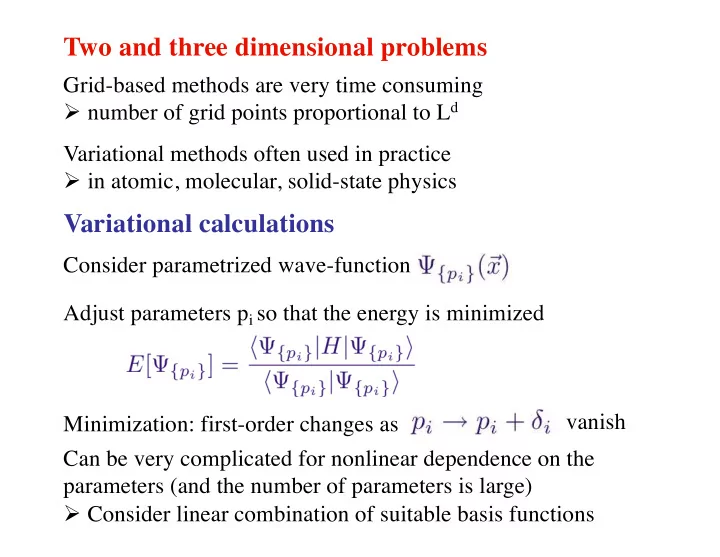
Two and three dimensional problems Grid-based methods are very time consuming Ø number of grid points proportional to L d Variational methods often used in practice Ø in atomic, molecular, solid-state physics Variational calculations Consider parametrized wave-function Adjust parameters p i so that the energy is minimized vanish Minimization: first-order changes as Can be very complicated for nonlinear dependence on the parameters (and the number of parameters is large) Ø Consider linear combination of suitable basis functions

Linear variational calculations Expansion in terms of a finite number of basis states Leads to a matrix eigenvalue problem if the basis is orthogonal Ø generalized eigenvalue problem for non-orthogonal basis Ø the energies are above the true energies (essence of “ variational ” ) Ø systematic improvements as size N of basis increased Ø basis states can be adapted to the potential under study First: Derivation of the matrix form of the Schrodinger equation

Another quantum mechanics refresher… Relation between abstract state and its wave function describes particle localized at delta-function overlap (scalar product) The wave function is the overlap with the position-basis states Expansion in a complete discrete set of orthonormal states position-dependent wave function in the k states

Expansion coefficients; wave function in k basis: If we have the real-space wave function, the coefficients are Example of discrete basis: Momentum state in periodic box: V = box volume. Expansion coefficients are Fourier transforms Allowed wave vectors (satisfying the periodic boundary conditions)

The matrix Schrodinger equation (any discrete basis) Schrodinger equation in general operator form Use expansion in discrete basis Rewrite H|k> as This gives Requires for each p (because of orthogonality)

Corresponds to matrix equation This is the Schrodinger equation in the k-basis Ø Solution: diagonalization of the Hamiltonian matrix Can be diagonalized numerically in finite basis Variational calculation • Chose “ good ” basis • Calculate matrix elements for p,k =1,...,N (truncated basis) • Diagonalize the matrix

Proof that the procedure is variational (minimizes E) Change in the coefficient Energy becomes (leading order) Can be written (leading order) as The linear shift in the energy is then

For this to vanish we must have H is hermitean -> Exactly the same condition as the matrix Schrodinger equation - Solution of the matrix Schrodeinger equation gives extremal (minimum) values of the energies for given basis size N - Increasing N cannot lead to higher energies, because setting C N+1 =0 gives same solution as before for C k , k=1,...,N - The energies must approach exact energies as N grows So, this is a variational procedure

Matrix diagonalization In principle, the secular equation gives eigenvalues of a matrix The eigenvectors i=1,...,N are obtained by solving Does not work well in practice (secular equation hard to solve) Methods exist for systematically finding transformation matrix Multiply by D from left; columns D n are the eigenvectors How to proceed in practice? Ø Read about it in Numerical Recipes or other numerics source Ø Use “ canned ” diagonalization routines - some (+ test codes) available on the course web site Ø Useful subroutine library: http://gams.nist.gov

Example of variational calculation 1D square well with central barrier Use eigenstates of pure square well (infinite walls) in variational calculation for the well with a square structure in the middle. These states are eigenstates of the kinetic energy; How do we approach the true solution as basis size N increases? Ø expect faster convergence for smaller V c

a=0.5 Ground state as a function of N Wave function N Energy 1 9.41680 3 7.98175 5 7.79671 7 7.78016 9 7.76888 11 7.76593 13 7.76365 15 7.76276 ... 25 7.76105 50 7.76062 true: 7.76056 (can be obtained using the Numerov + shooting method)

How about an asymmetric barrier? N energy 1 8.48449 2 6.01721 3 5.06098 4 5.01719 5 4.99315 6 4.96887 8 4.96195 10 4.95900 ... 20 4.95466 ... 50 4.95407 true: 4.95402

Let ’ s do a large barrier; V c =50 What ’ s going on? Ø No agreement N energy 2 29.93480 Ø Wrong symmetry? 4 14.86237 (comp with Numerov) 6 13.79536 8 13.62645 10 13.56317 ... 20 13.48853 30 13.47853 ... 100 13.47439 Numerov: 13.45011 (based on 10 8 steps)

Explanation Two almost degenerate states (symmetric/anti-symmetric) Ø Numerical accuracy problems; Numerov mixes them Ø The variational method easily keeps them separated (but larger errors in the energy) N=20 E0=13.4885 E1=13.4904 N=100 E0=13.4744 E1=13.4773 Numerov: 13.45011 (based on 10 8 steps)