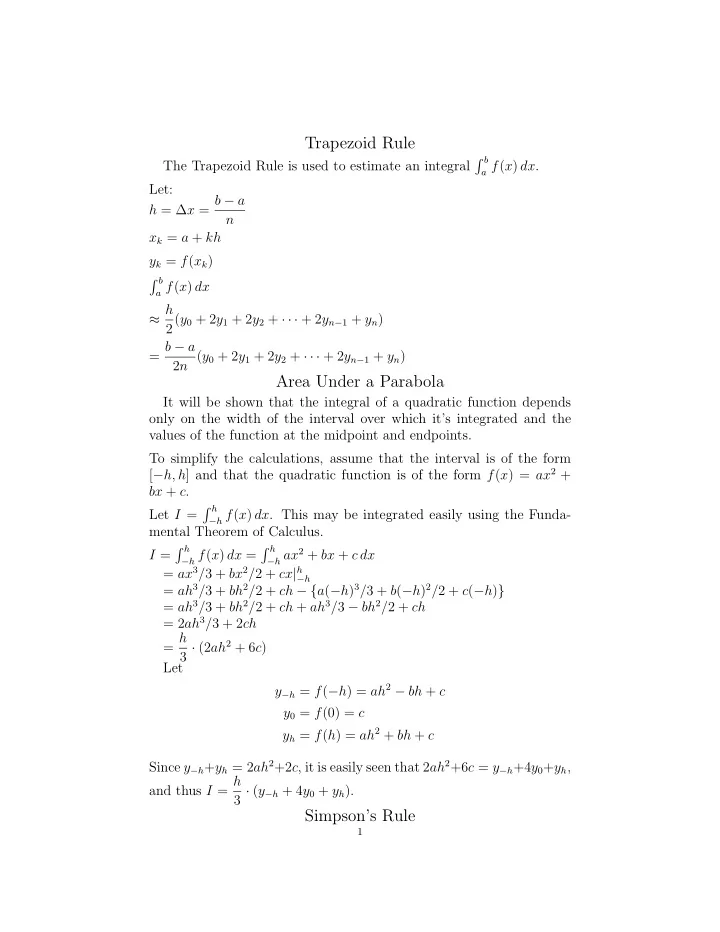
Trapezoid Rule b The Trapezoid Rule is used to estimate an integral - - PDF document

Trapezoid Rule

The Trapezoid Rule is used to estimate an integral b

a f(x) dx.

Let: h = ∆x = b − a n xk = a + kh yk = f(xk) b

a f(x) dx

≈ h 2(y0 + 2y1 + 2y2 + · · · + 2yn−1 + yn) = b − a 2n (y0 + 2y1 + 2y2 + · · · + 2yn−1 + yn)

Area Under a Parabola

It will be shown that the integral of a quadratic function depends

• nly on the width of the interval over which it’s integrated and the

values of the function at the midpoint and endpoints. To simplify the calculations, assume that the interval is of the form [−h, h] and that the quadratic function is of the form f(x) = ax2 + bx + c. Let I = h

−h f(x) dx. This may be integrated easily using the Funda-

mental Theorem of Calculus. I = h

−h f(x) dx =

h

−h ax2 + bx + c dx

= ax3/3 + bx2/2 + cx|h

−h

= ah3/3 + bh2/2 + ch − {a(−h)3/3 + b(−h)2/2 + c(−h)} = ah3/3 + bh2/2 + ch + ah3/3 − bh2/2 + ch = 2ah3/3 + 2ch = h 3 · (2ah2 + 6c) Let y−h = f(−h) = ah2 − bh + c y0 = f(0) = c yh = f(h) = ah2 + bh + c Since y−h+yh = 2ah2+2c, it is easily seen that 2ah2+6c = y−h+4y0+yh, and thus I = h 3 · (y−h + 4y0 + yh).

Simpson’s Rule

1

2

The Parabola Rule Simpson’s Rule may be used to approximate b

a f(x) dx. It takes the

idea of the Trapezoid Rule one degree higher. Rationale Partition the interval [a, b] evenly into n subintervals, where n is even, so that each subinterval has width h = b − a n and let yk = f(xk). Estimate the integral over adjacent pairs of integrals by the integral of a quadratic function agreeing with f at the midpoint and endpoints of the interval. x2

x0 f(x) dx ≈ h

3 · (y0 + 4y1 + y2) x4

x2 f(x) dx ≈ h

3 · (y2 + 4y3 + y4) x6

x4 f(x) dx ≈ h

3 · (y4 + 4y5 + y6) . . . xn

xn−2 f(x) dx ≈ h

3 · (yn−2 + 4yn−1 + yn) If everything is added together, we obtain the estimate b

a f(x) dx ≈ h

3 · (y0 + 4y1 + 2y2 + 4y3 + 2y4 + · · · + 2yn−2 + 4yn−1 + yn). This is known as Simpson’s Rule.

Summary

Midpoint Rule b

a f(x) dx ≈ h ·

• f

x0+x1

2

• + f

x1+x2

2

• + · · · + f

xn−1+xn

2

• Trapezoid Rule

b

a f(x) dx

≈ h 2(y0 + 2y1 + 2y2 + · · · + 2yn−1 + yn) = b − a 2n (y0 + 2y1 + 2y2 + · · · + 2yn−1 + yn) Simpson’s Rule b

a f(x) dx

≈ h 3 · (y0 + 4y1 + 2y2 + 4y3 + 2y4 + · · · + 2yn−2 + 4yn−1 + yn) = b − a 3n · (y0 + 4y1 + 2y2 + 4y3 + 2y4 + · · · + 2yn−2 + 4yn−1 + yn)

3

Error Estimates

Let ET be the error in the Trapezoid Rule. Let EM be the error in the Midpoint Rule. Let ES be the error in Simpson’s Rule. Let K be a bound on the second derivative. Let K∗ be a bound on the fourth derivative. |ET| ≤ K(b − a)3 12n2 |EM| ≤ K(b − a)3 24n2 |ES| ≤ K∗(b − a)5 180n4