Numerical integration example The probability that someones IQ falls - - PowerPoint PPT Presentation

Numerical integration example

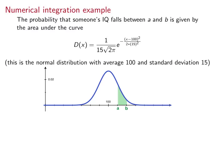
The probability that someone’s IQ falls between a and b is given by the area under the curve D(x) = 1 15 √ 2π e

− (x−100)2

2∗(15)2

(this is the normal distribution with average 100 and standard deviation 15)

100 0.02

a b

Numerical integration example

The probability that someone’s IQ falls between a and b is given by the area under the curve D(x) = 1 15 √ 2π e

(x−100)2

2∗(15)2

(this is the normal distribution with average 100 and standard deviation 15)

100 0.02

A

If someone has an IQ of A, they’re approximately in the percentile: Z A D(x)dx

( R 0

1 D(x)dx ≈ 0)

• Q. If you have an IQ of 130, what percentile are you in?

• Q. If you have an IQ of 130, what percentile are you in?

A. Z 130 1 15 √ 2π e

(x−100)2

2∗(15)2 dx

100 0.02

130

• Q. If you have an IQ of 130, what percentile are you in?

A. Z 130 1 15 √ 2π e

(x−100)2

2∗(15)2 dx ≈ 96.665%

Trapezoids with n = 8:

• Q. If you have an IQ of 130, what percentile are you in?

A. Z 130 1 15 √ 2π e

(x−100)2

2∗(15)2 dx ≈ 96.667%

Simpsons with n = 8:

How good are these estimates?

The error for each of these estimates can be bounded! Suppose you have approximated R b

a f (x) dx....

For Trapezoids, the error is bounded in terms of the second derivative of the function. For Simpson’s rule, the error is bounded in terms of the fourth derivative of the function.

How good are these estimates?

The error for each of these estimates can be bounded! Suppose you have approximated R b

a f (x) dx....

For Trapezoids, the error is bounded in terms of the second derivative of the function. error(n Trapezoids) ≤ M2(b − a)3/12 ∗ n2 where M2 is the maximum value of f 00(x) over the interval [a, b] For Simpson’s rule, the error is bounded in terms of the fourth derivative of the function. error(n subintervals, i.e. n

2 parabolas) ≤ M4(b − a)5/180 ∗ n4

where M4 is the maximum value of f (4)(x) over the interval [a, b]

f (x) = 1 15 √ 2π e

(x−100)2

2∗(15)2

f 00(x) = Ke1/450(x100)2(x2 − 200x + 9775),

where K = 1 759375 √ 2π

100

• 8⋅10-5

8⋅10-5

M2 = 0.00005275

f (x) = 1 15 √ 2π e

(x−100)2

2∗(15)2

f 00(x) = Ke1/450(x100)2(x2 − 200x + 9775),

where K = 1 759375 √ 2π

100

• 8⋅10-5

8⋅10-5

M2 = 0.00005275 So, the error in the Trapezoid approximation of Z 130 1 15 √ 2π e

(x−100)2

2∗(15)2 dx

with 8 trapezoids can’t be any larger than 0.00005275 ∗ 1303/(12 ∗ 82) ≈ 0.1509

f (x) = 1 15 √ 2π e

− (x−100)2

2∗(15)2

f (4)(x) = Ke−1/450(x−100)2(86651875−3730000x +58650x2−400x3+x4),

where K = 1 38443359375 √ 2π

100

• 5⋅10-6

5⋅10-6

M4 = 0.000001576

f (x) = 1 15 √ 2π e

(x−100)2

2∗(15)2

f (4)(x) = Ke1/450(x100)2(86651875−3730000x +58650x2−400x3+x4),

where K = 1 38443359375 √ 2π

100

• 5⋅10-6

5⋅10-6

M4 = 0.000001576 So, the error in the Simpson’s approximation of Z 130 1 15 √ 2π e

(x−100)2

2∗(15)2 dx

with 8 subintervals, i.e. 4 parabolas, can’t be any larger than 0.000001576 ∗ 1305/(180 ∗ 84) ≈ 0.07937

Example

Suppose we approximated R 5

0 ln(x + 1) dx using

(a) Trapezoids with n = 3, and (b) Simpson’s rule with n = 2. Which is guaranteed to be the better approximation?

Example

Suppose we approximated R 5

0 ln(x + 1) dx using

(a) Trapezoids with n = 3, and (b) Simpson’s rule with n = 2. Which is guaranteed to be the better approximation? Strategy:

• 1. Calculate the second and fourth derivatives of f (x).
• 2. Maximize f 00(x) over the interval [0, 5]. Call its maximum value M2.
• 3. Plug M2, (b − a) and n into the error bound formula for Trapezoids.
• 4. Maximize f (4)(x) over the interval [0, 5].

Call its maximum value M4.

• 5. Plug M4, (b − a) and n into the error bound formula Simpson’s rule.
• 6. Compare.

Area between curves

11/16/2011

Areas Between Curves

We know that if f is a continuous nonnegative function on the interval [a, b], then R b

a f (x)dx is the area under the graph of f and

above the interval. Now suppose we are given two continuous functions, f (x) and g(x) so that g(x) ≤ f (x) for all x in the interval [a, b]. How do we find the area bounded by the two functions over that interval?

f = top function g = bottom function

a b

=

a b

−

a b

Area between f and g = Z b

a

f (x)dx− Z b

a

g(x)dx = Z b

a

f (x)−g(x)dx

f = top function g = bottom function

a b

Area > 0

=

a b

(small negative)

−

a b

(bigger negative)

Area between f and g = Z b

a

f (x)dx− Z b

a

g(x)dx = Z b

a

f (x)−g(x)dx

f = top function g = bottom function

a b

Area > 0

=

a b

−

a b

(neg integral)

Area between f and g = Z b

a

f (x)dx− Z b

a

g(x)dx = Z b

a

f (x)−g(x)dx

Example

Find the area of the region between the graphs of y = x2 and y = x3 for 0 ≤ x ≤ 1.

1 1

Example

Find the area of the region between the graphs of y = x2 and y = x3 for 0 ≤ x ≤ 1.

1 1

Top: x2 Bottom: x3

Example

Find the area of the region between the graphs of y = x2 and y = x3 for 0 ≤ x ≤ 1.

1 1

Top: x2 Bottom: x3 Intersections: where does x2 = x3?

Example

Find the area of the region between the graphs of y = x2 and y = x3 for 0 ≤ x ≤ 1.

1 1

Top: x2 Bottom: x3 Intersections: where does x2 = x3? x = 0 or 1

Example

Find the area of the region between the graphs of y = x2 and y = x3 for 0 ≤ x ≤ 1.

1 1

Top: x2 Bottom: x3 Intersections: where does x2 = x3? x = 0 or 1 So Area = Z 1 x2−x3dx

Example

Find the area of the region between the graphs of y = x2 and y = x3 for 0 ≤ x ≤ 1.

1 1

Top: x2 Bottom: x3 Intersections: where does x2 = x3? x = 0 or 1 So Area = Z 1 x2−x3dx = 1 3x3−1 4x4

• 1

x=0 =

1

3 − 1 4

• − 0 > 0X

Example

Find the area of the region between y = ex and y = 1/(1 + x) on the interval [0, 1].

1 1 2

• 1. Check for intersection points (verify algebraically that x = 0 is

the only intersection by setting ex =

1 x+1).

• 2. Decide which function is on top (f (x)) and which function is
• n bottom (g(x)).
• 3. Calculate

R 1

0 f (x) − g(x)dx.

Check: What if you get a negative answer?

Example

Find the area of the region bounded by y = x2 − 2x and y = 4 − x2.

• 1. Check for intersection points (Solve x2 − 2x = 4 − x2). There

will be two, a and b; this is where the functions cross.

• 2. Between this two points, which function is on top (f (x)) and

which function is on bottom (g(x)).

• 3. Calculate

R b

a f (x) − g(x)dx.

Check: What if you get a negative answer?

Example

Find the area of the region bounded by y = x2 − 2x and y = 4 − x2.

• 1. Check for intersection points (Solve x2 − 2x = 4 − x2). There

will be two, a and b; this is where the functions cross.

• 2. Between this two points, which function is on top (f (x)) and

which function is on bottom (g(x)).

• 3. Calculate

R b

a f (x) − g(x)dx.

Check: What if you get a negative answer?

• 1

1 2

• 1

1 2 3 4

Example

Find the area of the region bounded by the two curves y = x3 − 9x and y = 9 − x2.

• 1. Check for intersection points (Solve x3 − 9x = 9 − x2).

Example

Find the area of the region bounded by the two curves y = x3 − 9x and y = 9 − x2.

• 1. Check for intersection points (Solve x3 − 9x = 9 − x2).
• 3
• 2
• 1

1 2 3

• 10
• 5

5 10

9"#"x^2 x^3"#"9x A B

Example

Find the area of the region bounded by the two curves y = x3 − 9x and y = 9 − x2.

• 1. Check for intersection points (Solve x3 − 9x = 9 − x2).
• 3
• 2
• 1

1 2 3

• 10
• 5

5 10

9"#"x^2 x^3"#"9x A B

• 2. Area = Area A + Area B

Example

Find the area of the region bounded by the two curves y = x3 − 9x and y = 9 − x2.

• 1. Check for intersection points (Solve x3 − 9x = 9 − x2).
• 3
• 2
• 1

1 2 3

• 10
• 5

5 10

9"#"x^2 x^3"#"9x A B

• 2. Area = Area A + Area B

Area A = Z −1

−3

(x3−9x)−(9−x2)dx = Z −1

−3

x3+x2−9x−9 dx

Example

Find the area of the region bounded by the two curves y = x3 − 9x and y = 9 − x2.

• 1. Check for intersection points (Solve x3 − 9x = 9 − x2).
• 3
• 2
• 1

1 2 3

• 10
• 5

5 10

9"#"x^2 x^3"#"9x A B

• 2. Area = Area A + Area B

Area A = Z −1

−3

(x3−9x)−(9−x2)dx = Z −1

−3

x3+x2−9x−9 dx Area B = Z 3

−1

(9−x2)−(x3−9x)dx = − Z 3

−1

x3+x2−9x−9 dx

Example

Find the area between sin x and cos x on [−3π/4, 5π/4].

• 2
• 1

1 2 3 4

sin(x) cos(x) A B

Functions of y

We could just as well consider two functions of y, say, x = fLeft(y) and x = gRight(y) defined on the interval [c, d].

Area Between the Two Curves

Find the area under the graph of y = ln x and above the interval [1, e] on the x-axis.

1 2 3 1 2 3

y x y=ln(x) x=e

Area Between the Two Curves

Find the area under the graph of y = ln x and above the interval [1, e] on the x-axis.

1 2 3 1 2 3

y x y=ln(x) x=e

1 2 3 1 2 3

y x x=e^y x=e