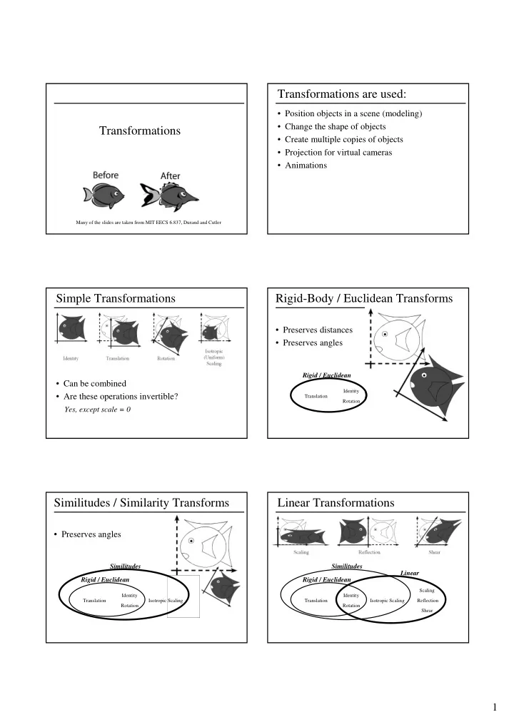
Transformations are used: Position objects in a scene (modeling) - - PDF document

transformations are used
SMART_READER_LITE
LIVE PREVIEW

Transformations are used: Position objects in a scene (modeling) - - PDF document

Transformations are used: Position objects in a scene (modeling) Change the shape of objects Transformations Create multiple copies of objects Projection for virtual cameras Animations Many of the slides are taken from MIT


slide-1
SLIDE 1

1

Transformations

Many of the slides are taken from MIT EECS 6.837, Durand and Cutler

Transformations are used:

  • Position objects in a scene (modeling)
  • Change the shape of objects
  • Create multiple copies of objects
  • Projection for virtual cameras
  • Animations

Simple Transformations

  • Can be combined
  • Are these operations invertible?

Yes, except scale = 0

Rigid-Body / Euclidean Transforms

  • Preserves distances
  • Preserves angles

Translation Rotation

Rigid / Euclidean

Identity

Similitudes / Similarity Transforms

  • Preserves angles

Translation Rotation

Rigid / Euclidean Similitudes

Isotropic Scaling Identity

Linear Transformations

Translation Rotation

Rigid / Euclidean Linear Similitudes

Isotropic Scaling Identity Scaling Shear Reflection

slide-2
SLIDE 2

2

Linear Transformations

  • L(p + q) = L(p) + L(q)
  • L(ap) = a L(p)

Translation Rotation

Rigid / Euclidean Linear Similitudes

Isotropic Scaling Scaling Shear Reflection Identity

Affine Transformations

  • preserves

parallel lines

Translation Rotation

Rigid / Euclidean Linear Similitudes

Isotropic Scaling Scaling Shear Reflection Identity

Affine

Projective Transformations

  • preserves lines

Translation Rotation

Rigid / Euclidean Linear Affine Projective Similitudes

Isotropic Scaling Scaling Shear Reflection Perspective Identity

Perspective Projection Outline

  • Assignment 0 Recap
  • Intro to Transformations
  • Classes of Transformations
  • Representing Transformations
  • Combining Transformations
  • Change of Orthonormal Basis

How are Transforms Represented?

x’ = ax + by + c y’ = dx + ey + f x’ y’ a b d e c f = x y +

p’ = M p + t

slide-3
SLIDE 3

3

Homogeneous Coordinates

  • Add an extra dimension
  • in 2D, we use 3 x 3 matrices
  • In 3D, we use 4 x 4 matrices
  • Each point has an extra value, w

x’ y’ z’ w’ = x y z w a e i m b f j n c g k

  • d

h l p

p’ = M p

Homogeneous Coordinates

  • Most of the time w = 1, and we can ignore it
  • If we multiply a homogeneous coordinate

by an affine matrix, w is unchanged x’ y’ z’ 1 = x y z 1 a e i b f j c g k d h l 1

Homogeneous Visualization

  • Divide by w to normalize (homogenize)
  • W = 0?

w = 1 w = 2

(0, 0, 1) = (0, 0, 2) = … (7, 1, 1) = (14, 2, 2) = … (4, 5, 1) = (8, 10, 2) = …

Point at infinity (direction)

3D Coordinate Systems

  • Right-handed coordinate system:
  • Left-handed coordinate system:

y z x x y z

3D Transformations

  • In homogeneous coordinates, 3D

transformations are represented by 4x4 matrices.

  • A point transformation is performed:
  • 1

1 1 ’ ’ ’ z y x t i h g t f e d t c b a z y x

z y x

Translate (tx, ty, tz)

  • Why bother with the

extra dimension?

Because now translations can be encoded in the matrix!

x’ y’ z’ = x y z 1 1 1 1 tx ty tz 1

Translate(c,0,0)

x y p p’

c

x’ y’ z’ 1

slide-4
SLIDE 4

4

Scale (sx, sy, sz)

  • Isotropic (uniform)

scaling: sx = sy = sz x’ y’ z’ 1 = x y z 1 sx sy sz 1

Scale(s,s,s)

x p p’ q q’ y

3D Shearing

  • The change in each coordinate is a linear combination of all

three.

  • Transforms a cube into a general parallelepiped.
  • 1

1 1 1 1 1 z fy ex dz y cx bz ay x z y x f e d c b a

Rotation

  • About z axis

x’ y’ z’ 1 = x y z 1 cos sin

  • sin

cos 1 1

ZRotate( )

x y z p p’

Rotation

  • About

x axis:

  • About

y axis: x’ y’ z’ 1 = x y z 1 cos sin

  • sin

cos 1 1 x’ y’ z’ 1 = x y z 1 cos

  • sin

sin cos 1 1 1

Rotation

  • About (kx, ky, kz), a unit

vector on an arbitrary axis (Rodrigues Formula) x’ y’ z’ 1 = x y z 1 kxkx(1-c)+c kykx(1-c)+kzs kzkx(1-c)-kys 1 kzkx(1-c)-kzs kzkx(1-c)+c kzkx(1-c)-kxs kxkz(1-c)+kys kykz(1-c)-kxs kzkz(1-c)+c

where c = cos & s = sin

Rotate(k, )

x y z

k

3D Rotation

  • To generate a rotation in 3D we have to

specify:

– axis of rotation (2 d.o.f) – amount of rotation (1 d.o.f)

  • Note, the axis passes through the origin.

x y z

slide-5
SLIDE 5

5

A counter-clockwise rotation about the z-axis:

  • 1

1 1 cos sin sin cos 1 ’ ’ ’ z y x z y x

  • y

z x

p R p

z

) ( ’

  • A counter-clockwise rotation about the x-axis:
  • 1

1 cos sin sin cos 1 1 ’ ’ ’ z y x z y x

  • y

z x

p R p

x

) ( ’

  • A counter-clockwise rotation about the y-axis:
  • 1

1 cos sin 1 sin cos 1 ’ ’ ’ z y x z y x

  • y

z x

p R p

y

) ( ’

  • Inverse Rotation

’ ) ( ’ ) (

1

p R p R p

  • Composite Rotations
  • Rx, Ry, and Rz, can perform any rotation about an

axis passing through the origin.

About Rotations

Rotation About an Arbitrary Axis

  • Axis of rotation can be located at any point: 6 d.o.f.
  • The idea: make the axis coincident with one of the

coordinate axes (z axis), rotate, and then transform back.

  • Assume that the axis passes through the point p0.

y z x

p0

  • Steps:

– Translate P0 to the origin. – Make the axis coincident with the z-axis (for example):

  • Rotate about the x-axis into the xz plane.
  • Rotate about the y-axis onto the z-axis.
  • Rotate as needed about the z-axis.
  • Apply inverse rotations about y and x.
  • Apply inverse translation.

Rotation About an Arbitrary Axis

slide-6
SLIDE 6

6

y z x

p0

A

y x

p0

z

B

y x

p0

z

C

y x

p0

z y x

p0

z

E

y z x

p0

F

Rotation About an Arbitrary Axis Outline

  • Assignment 0 Recap
  • Intro to Transformations
  • Classes of Transformations
  • Representing Transformations
  • Combining Transformations
  • Change of Orthonormal Basis

How are transforms combined?

(0,0) (1,1) (2,2) (0,0) (5,3) (3,1) Scale(2,2) Translate(3,1)

TS =

2 2 1 1 3 1 2 2 3 1

= Scale then Translate Use matrix multiplication: p' = T ( S p ) = TS p Caution: matrix multiplication is NOT commutative!

0 0 1 0 0 1 0 0 1

Non-commutative Composition

Scale then Translate: p' = T ( S p ) = TS p Translate then Scale: p' = S ( T p ) = ST p

(0,0) (1,1) (4,2) (3,1) (8,4) (6,2) (0,0) (1,1) (2,2) (0,0) (5,3) (3,1) Scale(2,2) Translate(3,1) Translate(3,1) Scale(2,2)

TS =

2 2 1 1 1 3 1 1

ST =

2 2 1 1 3 1

Non-commutative Composition

Scale then Translate: p' = T ( S p ) = TS p

2 2 3 1 1 2 2 6 2

= = Translate then Scale: p' = S ( T p ) = ST p

0 0 1 0 0 1 0 0 1

Outline

  • Assignment 0 Recap
  • Intro to Transformations
  • Classes of Transformations
  • Representing Transformations
  • Combining Transformations
  • Change of Orthonormal Basis
slide-7
SLIDE 7

7

Review of Dot Product

b a

Change of Orthonormal Basis

  • Given:

coordinate frames xyz and uvn point p = (x,y,z)

  • Find:

p = (u,v,n)

p x y z v u x y v u n p x y u v

Change of Orthonormal Basis

(x . u) u (y . u) u (z . u) u (x . v) v (y . v) v (z . v) v (x . n) n (y . n) n (z . n) n x y z = = = + + + + + +

x y z v u n x . u x . v y . v y . u x y v u

Change of Orthonormal Basis

(x . u) u (y . u) u (z . u) u (x . v) v (y . v) v (z . v) v (x . n) n (y . n) n (z . n) n x y z = = = + + + + + + p = (x,y,z) = x x + y y + z z (x . u) u (y . u) u (z . u) u (x . v) v (y . v) v (z . v) v (x . n) n (y . n) n (z . n) n + + + + + + x [ y [ z [ ] + ] + ] Substitute into equation for p: p =

Change of Orthonormal Basis

(x . u) u (y . u) u (z . u) u (x . v) v (y . v) v (z . v) v (x . n) n (y . n) n (z . n) n p = + + + + + + x [ y [ z [ ] + ] + ] x (x . u) x (x . v) x (x . n) y (y . u) y (y . v) y (y . n) z (z . u) z (z . v) z (z . n) + + + + + + [ [ [ ] u + ] v + ] n Rewrite: p =

Change of Orthonormal Basis

x (x . u) x (x . v) x (x . n) u v n = = = + + + + + + y (y . u) y (y . v) y (y . n) z (z . u) z (z . v) z (z . n) p = x (x . u) x (x . v) x (x . n) y (y . u) y (y . v) y (y . n) z (z . u) z (z . v) z (z . n) + + + + + + [ [ [ ] u + ] v + ] n p = (u,v,n) = u u + v v + n n Expressed in uvn basis:

slide-8
SLIDE 8

8

Change of Orthonormal Basis

u v n = x y z ux vx nx uy vy ny uz vz nz x (x . u) x (x . v) x (x . n) u v n = = = + + + + + + y (y . u) y (y . v) y (y . n) z (z . u) z (z . v) z (z . n) In matrix form:

ux = x . u where: etc. uy = y . u

Change of Orthonormal Basis

u v n = x y z ux vx nx uy vy ny uz vz nz What’ s M-1, the inverse?

ux = x . u = u . x = xu

u v n = x y z xu yu zu xv yv zv xn yn zn = M x y z

M-1 = MT

Changing Coordinate Systems

u=(ux,uy,uz) v=(vx,vy,vz) w=(wx,wy,wz)

(x0,y0,z0)

y z x

M is rotation matrix whose columns are U,V, and W:

U u u u w v u w v u w v u MX

z y x z z z y y y x x x

  • 1

1 1 1

And the inverse…

X u u u u u u w w w v v v u u u U M

z y x z y x z y x z y x z y x T

  • 1

1 1 1 1

2 2 2

For the rotation matrix:

1

  • R

RT

Transforming Planes

  • Plane representation:

– By three non-collinear points – By implicit equation:

  • 1
  • z

y x D C B A D Cz By Ax

P0 P1 P2

  • 1

z y x

  • 1

D C D B D A

slide-9
SLIDE 9

9

Transforming Planes

  • One way to transform a plane is by transforming any three non-collinear

points on the plane.

  • Another way is to transform the plane equation: Given a transformation T

that transforms [x,y,z,1] to [x’,y’,z’,1] find [A',B',C',D'], such that:

  • 1

1

  • z

y x T T D C B A

  • 1

’ ’ ’ ’ ’ ’ ’

  • z

y x D C B A

  • D

C B A T D C B A

T 1

’ ’ ’ ’

T T

AT A AT A ) ( ) ’ ( ’

1 1