TRANSFERRING DIFFUSION BASED MANIFOLD C Diffusion Maps Embryoid - - PowerPoint PPT Presentation

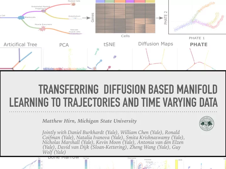
tem Cell Myeloid Cells Endothelium Vascular muscle cells Blastocysts Muscle Precursors Endothelial-Myeloid Progenitors

Cells Genes

PHATE 1 PHATE 2

B

PHATE tSNE Diffusion Maps PCA Articifical Tree

C

PHATE tSNE Diffusion Maps PCA Embryoid Bodies

D

Prevotella Firmicutes

CyTOF iPSC MARS-seq Bone Marrow Hi-C Gut Microbiome Facebook

TRANSFERRING DIFFUSION BASED MANIFOLD LEARNING TO TRAJECTORIES AND TIME VARYING DATA

Matthew Hirn, Michigan State University Jointly with Daniel Burkhardt (Yale), William Chen (Yale), Ronald Coifman (Yale), Natalia Ivanova (Yale), Smita Krishnaswamy (Yale), Nicholas Marshall (Yale), Kevin Moon (Yale), Antonia van den Elzen (Yale), David van Dijk (Sloan-Kettering), Zheng Wang (Yale), Guy Wolf (Yale)

MANIFOLD LEARNING

• Data X = {x1, . . . , xn} ⇢ (M, g) ,

! Rd sampled iid from some distribution

• Extrinsic dimension d possibly large: dim(M) ⌧ d
• How do we obtain new coordinates X 7! Y = {y1, . . . , yn} ⇢ Rk with

k ⇠ dim(M) that preserve the underlying local geometry?

• Cam we simultaneously emphasize clusters within the data?

n

MANIFOLD LEARNING

• Data X = {x1, . . . , xn} ⇢ (M, g) ,

! Rd sampled iid from some distribution

• Extrinsic dimension d possibly large: dim(M) ⌧ d
• How do we obtain new coordinates X 7! Y = {y1, . . . , yn} ⇢ Rk with

k ⇠ dim(M) that preserve the underlying local geometry?

• Cam we simultaneously emphasize clusters within the data?

n

MANIFOLD LEARNING

First coordinate of embedding

• Data X = {x1, . . . , xn} ⇢ (M, g) ,

! Rd sampled iid from some distribution

• Extrinsic dimension d possibly large: dim(M) ⌧ d
• How do we obtain new coordinates X 7! Y = {y1, . . . , yn} ⇢ Rk with

k ⇠ dim(M) that preserve the underlying local geometry?

• Cam we simultaneously emphasize clusters within the data?

n

DIFFUSION MAPS

Coifman, Lafon 2006 Nadler, Lafon, Coifman, Kevrekidis, 2006

• Local similarity kernel: Kij = k(xi, xj) = e≠Îxi≠xjÎ2/‘
• Sampling density estimate: Qii = q

j Kij

• Density normalization: Â

K = Q≠–KQ≠– ¶ α = 0 ∆ full influence of sampling statistics ¶ α = 1

2 ∆ stochastic differential equations

¶ α = 1 ∆ geometry only, no sampling bias (used in this talk)

• One more normalization: Dii = q

j Â

Kij

• Random walk: P = P‘ = D≠1 Â

K

DIFFUSION MAPS

Coifman, Lafon 2006 Heat equation: ∂tu = ∆u

• Define the diffusion distance as:

Dt(xi, xj)2 =

n

ÿ

l=1

(P t

il − P t jl)2 1

πl

• Theorem [CL06]: For α = 1 (assumed from here forward),

lim

n→∞ ‘→0

P t/‘

‘

= et∆ (the heat kernel)

DIFFUSION MAPS

Coifman, Lafon 2006 Heat equation: ∂tu = ∆u

• Define the diffusion distance as:

Dt(xi, xj)2 =

n

ÿ

l=1

(P t

il − P t jl)2 1

πl

• Theorem [CL06]: For α = 1 (assumed from here forward),

lim

n→∞ ‘→0

P t/‘

‘

= et∆ (the heat kernel)

DIFFUSION MAPS

B´ erard, Besson, Gallot 1994 Coifman, Lafon 2006

Truncated to give low dimensional embedding

• Let 1 = λ0 > λ1 Ø · · · Ø λn−1 Ø 0 be the eigenvalues of P,

with eigenvectors 1 = ψ0, ψ1, . . . , ψn−1.

• Define the diffusion map:

Ψt(xi) = (λt

1ψ1(xi), . . . , λt n−1ψn−1(xi))

• Theorem [BBG94, CL06]: The diffusion distance satisfies:

Dt(xi, xj) = ÎΨt(xi) ≠ Ψt(xj)Î

• Theorem [BBG94]: If we compute Ψt using the heat kernel, the pulled back

metric Ψ∗

t is asymptotic to the metric g of M when t æ 0+

OUTLINE

• Non-manifold data: Metric trees, biology and PHATE
• Time varying data: Time coupled diffusion maps and condensation
• Future directions and conclusions

Stem Cell Myeloid Cells Endothelium Vascular muscle cells Blastocysts Muscle Precursors Endothelial-Myeloid Progenitors

Non-manifold trajectory data

METRIC TREE EMBEDDINGS

Diffusion maps - what is happening here?

Moon, van Dijk, Wang, Burkhardt, Chen, van den Elzen, H., Coifman, Ivanova, Wolf, Krishnaswamy 2017

DIFFUSION MAPS AND METRIC TREES

Metric tree (colored by edge)

Diffusion maps embedding x 7! (ψi(x), ψj(x)) for i, j = 1, . . . , 10

ψi(x)

ψj(x) Moon, van Dijk, Wang, Burkhardt, Chen, van den Elzen, H., Coifman, Ivanova, Wolf, Krishnaswamy 2017

DIFFUSION MAPS AND METRIC TREES

Metric tree (colored by edge)

Eigenvector ψ1(x)

Moon, van Dijk, Wang, Burkhardt, Chen, van den Elzen, H., Coifman, Ivanova, Wolf, Krishnaswamy 2017

DIFFUSION MAPS AND METRIC TREES

Metric tree (colored by edge)

Eigenvector ψ2(x)

Moon, van Dijk, Wang, Burkhardt, Chen, van den Elzen, H., Coifman, Ivanova, Wolf, Krishnaswamy 2017

DIFFUSION MAPS AND METRIC TREES

Metric tree (colored by edge)

Eigenvector ψ3(x)

Moon, van Dijk, Wang, Burkhardt, Chen, van den Elzen, H., Coifman, Ivanova, Wolf, Krishnaswamy 2017

DIFFUSION MAPS AND METRIC TREES

Metric tree (colored by edge)

Eigenvector ψ4(x)

Moon, van Dijk, Wang, Burkhardt, Chen, van den Elzen, H., Coifman, Ivanova, Wolf, Krishnaswamy 2017

DIFFUSION MAPS AND METRIC TREES

Metric tree (colored by edge)

Eigenvector ψ5(x)

Moon, van Dijk, Wang, Burkhardt, Chen, van den Elzen, H., Coifman, Ivanova, Wolf, Krishnaswamy 2017

DIFFUSION MAPS AND METRIC TREES

Metric tree (colored by edge)

Eigenvector ψ6(x)

Moon, van Dijk, Wang, Burkhardt, Chen, van den Elzen, H., Coifman, Ivanova, Wolf, Krishnaswamy 2017

DIFFUSION MAPS AND METRIC TREES

Metric tree (colored by edge)

Eigenvector ψ7(x)

Moon, van Dijk, Wang, Burkhardt, Chen, van den Elzen, H., Coifman, Ivanova, Wolf, Krishnaswamy 2017

DIFFUSION MAPS AND METRIC TREES

Metric tree (colored by edge)

Eigenvector ψ8(x)

Moon, van Dijk, Wang, Burkhardt, Chen, van den Elzen, H., Coifman, Ivanova, Wolf, Krishnaswamy 2017

DIFFUSION MAPS AND METRIC TREES

Metric tree (colored by edge)

Eigenvector ψ9(x)

Moon, van Dijk, Wang, Burkhardt, Chen, van den Elzen, H., Coifman, Ivanova, Wolf, Krishnaswamy 2017

DIFFUSION MAPS AND METRIC TREES

Metric tree (colored by edge)

Eigenvector ψ10(x)

Moon, van Dijk, Wang, Burkhardt, Chen, van den Elzen, H., Coifman, Ivanova, Wolf, Krishnaswamy 2017

DIFFUSION MAPS AND METRIC TREES

Metric tree (colored by edge)

Eigenvector ψ10(x)

Conjecture: To embed the tree with diffusion maps as x 7! (ψi1(x), . . . , ψik(x)), need k ⇠ depth of the tree Punchline: The information is there, but we need a different way to get at it

Moon, van Dijk, Wang, Burkhardt, Chen, van den Elzen, H., Coifman, Ivanova, Wolf, Krishnaswamy 2017

GEOMETRY AND TIME SCALES

• Theorem [Varadhan 1967]: Small time diffusions preserve geometry. Let

K(t, x, x0) be the heat kernel on M. Then: lim

t!0+ t log K(t, x, x0) = −1

4r(x, x0)2

• Numerically, though, this is perilous
• However, on M = Rd, we have K(t, x, x0) =

1 (4πt)d/2 exp(−|x − x0|2/4t),

and so in this case we have for all t > 0: t log K(t, x, x0) = −d 2t log(4πt) − 1 4|x − x0|2

• Metric trees lie somewhere in between these two regimes, so we propagate P t

for an intermediate value of t and compute: U (t) = U (t)

ij = t log P t ij

• We then apply multidimensional scaling (MDS) to the rows of U (t) to get the

PHATE embedding

• Open problem to make the above reasoning rigorous

Moon, van Dijk, Wang, Burkhardt, Chen, van den Elzen, H., Coifman, Ivanova, Wolf, Krishnaswamy 2017

BACK TO THE BINARY TREE

Metric tree (colored by edge)

PHATE embedding

Moon, van Dijk, Wang, Burkhardt, Chen, van den Elzen, H., Coifman, Ivanova, Wolf, Krishnaswamy 2017

STEM CELL DATA

Stem Cell Myeloid Cells Endothelium Vascular muscle cells

PHATE 1 PHATE 2 Cells Genes

Blastocysts Muscle Precursors Endothelial-Myeloid Progenitors

Moon, van Dijk, Wang, Burkhardt, Chen, van den Elzen, H., Coifman, Ivanova, Wolf, Krishnaswamy 2017

ESC Mesoderm NCC Prog. Neural Prog. Mix of Meso. and NCC Cardiac Prog. Neuroectoderm

PHATE

STEM CELL DATA

PCA

tSNE

Diffusion maps

Moon, van Dijk, Wang, Burkhardt, Chen, van den Elzen, H., Coifman, Ivanova, Wolf, Krishnaswamy 2017

MOUSE BEHAVIORAL DATA

OPEN QUESTIONS

• Can we develop rigorous mathematical theory relating diffusion geometry to

metric trees?

• If so, can these ideas in turn shed light on the more general problems of

intersecting hyperplanes or intersecting manifolds?

• All of these directions are potentially relevant for the topics in the remainder
• f this talk

Time varying manifold data

TIME VARYING DATA MODEL

t = 1 t = 20 t = 40 t = 60 t = 80 t = 100 t = 120 t = 140 t = 160 t = 180

Marshall, H. 2017

What about time varying data but with minimal assumptions on the data generation process?

• Manifold model: Compact Riemannian manifold (M, g(t)) with smoothly

varying metric g(t)

• New heat equation:

∂tu = ∆g(t)u (couples heat diffusion with changing geometry)

• Theorem [Guenther 2002]: There exists a fundamental solution (heat ker-

nel) Z(x, t; x0, s) for the above heat equation.

TIME COUPLED DIFFUSION MAP

Marshall, H. 2017

t1, . . . , tm

(M, g(t))

• We want to approximate the integral operator associated to Z:

T (t)

Z f(x) =

Z

M

Z(x, t; x0, 0)f(x0) dV (x0, 0)

• Data: Time samples 0 = t1 < t2 < · · · < tm = t and manifold samples at

each time, Xk = {x1(tk), . . . , xn(tk)} ⊂ (M, g(t)) , → Rd

• For each time tk, approximate the heat diffusion over (M, g(t)) from time tk

to tk+1 with one step of the random walk P✏,tk, which is computed on the data Xk

• Define an m-step time inhomogeneous random walk up to time tm = t as:

P (m)

✏

= P✏,tmP✏,tm−1 · · · P✏,1

• Theorem: The inhomogeneous random walk approximates T (t)

Z :

lim

n→∞ ✏→0

P (t/✏)

✏

= T (t)

Z

• A time coupled diffusion map is defined in terms of the SVD of P (m)

✏

DEFORMED BAR BELL

Marshall, H. 2017

t = start

t = end t = middle

CONDENSATION

We can also drive the changing metric ourselves:

• Recall data X = X0 = {x1, . . . , xn} ⊂ Rd
• Suppose xi = x(0)

i

= (f1(xi), . . . , fd(xi)) so that fj ∈ Rn

• Let P1 ∈ Rn×n be the diffusion operator generated from X0
• Define x(1)

i

= (P1f1(xi), . . . , P1fd(xi)), which gives a data set X1 = {x(1)

1 , . . . , x(1) n }

• Iterate the process yielding:

x(m)

i

= (Pm · · · P1f1(xi), . . . , Pm · · · P1fd(xi)) Pk = Diffusion operator generated from Xk−1

• Yields multiscale cluster progressions

Welp, Wolf, H., Krishnaswamy 2016

• C. ELEGANS NEURONS

Sankey diagram of the condensation history of C. Elegans neurons. The neurons are grouped into progressively more associated groups, the colors represent the final cluster assignment.

Welp, Wolf, H., Krishnaswamy (in progress)

OPEN QUESTIONS

• We know the inhomogeneous Markov chain approximates T (t)

Z , but what is

the precise nature of the joint spatial-temporal geometric information encoded by the SVD of this operator?

• Can we say anything mathematically precise about the condensation process?
• More generally, are there other ways to manipulate the geometry of data and

interpret it via this type of analysis?

• What if we do not have a bijective correspondence between spatial samples
• ver time?

CONCLUSIONS

• New geometric models for increasingly complex data require new mathemat-

ical understanding in order to best analyze such data and avoid spurious sci- entific conclusions (e.g., metric trees, time varying data and inhomogeneous random walks)

• The underlying tool for the work presented here is diffusion based manifold

learning

• However, to push beyond the existing boundaries of this field, new and more

flexible ideas are needed