
SLIDE 1
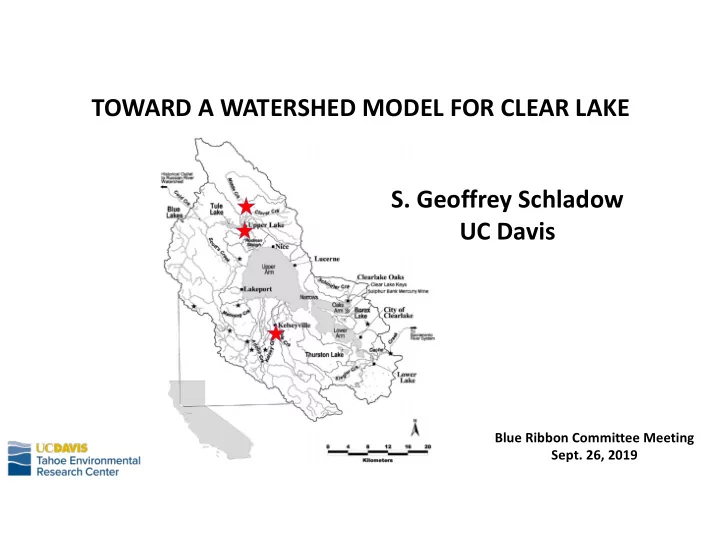
TOWARD A WATERSHED MODEL FOR CLEAR LAKE
- S. Geoffrey Schladow
UC Davis
Blue Ribbon Committee Meeting
- Sept. 26, 2019
TOWARD A WATERSHED MODEL FOR CLEAR LAKE S. Geoffrey Schladow UC - - PowerPoint PPT Presentation
TOWARD A WATERSHED MODEL FOR CLEAR LAKE S. Geoffrey Schladow UC Davis Blue Ribbon Committee Meeting Sept. 26, 2019 A distributed watershed model is a computer model that uses sets of mathematical equations to: 1. Simulate hydrologic processes
Lake Tahoe
Elevation 1889 - 2044 2045 - 2200 2201 - 2356 2357 - 2512 2513 - 2667 2668 - 2823 2824 - 2979 2980 - 3135 3136 - 3291 No Data Lake Tahoe Subwatersheds
1 2 3 4 5 Kilometers
Subwatersheds Streams Lake Tahoe
N
Watersheds
Lake Tahoe
N
Lake Tahoe Final Composite Land Use Residential_SFP Residential_MFP CICU-Pervious Ski Runs-Pervious Vegetation-Unimpacted Vegetation-Recreational Vegetation-Turf Waterbody Roads-Unpaved Residential_SFI Residential-MFI CICU-Impervious Roads-Primary Roads-Secondary Subwatersheds
10 20 Miles
Countless uses of satellite data
movement etc.
5 kilometers
Erodibility classes 1 2 3 4 5
Pervious/Impervious Subcategory Name
Pervious SFR - Pervious Impervious SFR - Impervious Pervious MFR - Pervious Impervious MFR - Impervious Pervious CICU - Pervious Impervious CICU - Impervious Impervious Primary Roads Impervious Secondary Roads Pervious Unpaved Roads Pervious Ski Runs Pervious Recreation Pervious Burned Pervious Harvest Pervious Turf Areas Pervious Erosion Potential - 1 Pervious Erosion Potential - 2 Pervious Erosion Potential - 3 Pervious Erosion Potential - 4 Pervious Erosion Potential - 5
Transportation Vegetated Single Family Residential Multi Family Residential Commercial/Institutional/ Communications/Utilities
10 20 30 40 50 60 70 80 1/1/1995 7/1/1995 1/1/1996 7/1/1996 1/1/1997 7/1/1997 1/1/1998 7/1/1998 1/1/1999 7/1/1999 1/1/2000 7/1/2000 1/1/2001 7/1/2001 1/1/2002 7/1/2002 1/1/2003 7/1/2003 1/1/2004 7/1/2004 1/1/2005 Average Temperature (Deg F) 3 6 9 12 15 18 21 24 Data Quality (Impaired Hours) Number of Impaired Hours per Day Original Hourly SNOTEL Temperature (Fallen Leaf) Corrected Temperature * Historical average monthly reference crop evapotranspiration for Tahoe City, California UC Davis Division of Agriculture and Natural Resources, Publication 21454 1 2 3 4 5 6 7 8 Jan Feb Mar Apr May Jun Jul Aug Sep Oct Nov Dec Inches/Month Tahoe City Reference ET * Reference ET adjusted for Evergreen Forest LSPC Modeled Total ET (10/1996-9/2003)
% U % U % U % U % U % U % U % U % U ( X ( X ( X
Lake Tahoe
SKI AREA TAHOE CITY CROSS WARD CREEK MARLETTE LAKE RUBICON FALLEN LEAF ECHO PEAK HAGAN'S MEADOW HEAVENLY VALLEY GLENBROOK DAGGET PASS SOUTH LAKE TAHOE AP N
Subwatersheds Lake Tahoe
% U
NRCS SNOTEL Stations
( X
NCDC Weather Stations
10 20 Miles
% U % U % U % U % U % U % U % U % U % U % U % U % U
# Y # Y # Y # Y # Y # Y # Y # Y # Y # Y
Lake Tahoe Third Creek Incline Creek Ward Creek Blackwood Creek General Creek Marlette Creek Glenbrook Creek Logan House Creek Edgewood Creek Upper Truckee River at South Lake Tahoe Trout Creek Upper Truckee River at Hwy 50 Upper Truckee River at S. Upper Truckee Road
N
Subwatersheds Streams Lake Tahoe
% U
USGS Flow Gages
# Y
LTIMP Water Quality Stations
10 20 Miles
1,000 2,000 3,000 4,000 5,000 6,000 7,000 R e s i d e n t i a l _ S F P R e s i d e n t i a l _ M F P C I C U
e r v i
s S k i _ R u n s
e r v i
s V e g _ e p 1 V e g _ e p 2 V e g _ e p 3 V e g _ e p 4 V e g _ e p 5 V e g _ R e c r e a t i
a l V e g _ B u r n e d V e g _ H a r v e s t V e g _ T u r f W a t e r _ B
y R e s i d e n t i a l _ S F I R e s i d e n t i a l _ M F I C I C U
m p e r v i
s R
d s _ P r i m a r y R
d s _ S e c
d a r y R
d s _ U n p a v e d Load, MT/yr Upland Fines, metric tons Upland TSS, metric tons
1,000 2,000 3,000 4,000 5,000 6,000 Residential_SFP Residential_MFP CICU-Pervious Ski_Runs-Pervious Veg_ep1 Veg_ep2 Veg_ep3 Veg_ep4 Veg_ep5 Veg_Recreational Veg_Burned Veg_Harvest Veg_Turf Water_Body Residential_SFI Residential_MFI CICU-Impervious Roads_Primary Roads_Secondary Roads_Unpaved Load, kg/yr
Surface TP, kg/yr Baseflow TP, kg/yr
5,000 10,000 15,000 20,000 25,000 30,000 R e s i d e n t i a l _ S F P R e s i d e n t i a l _ M F P C I C U
e r v i
s S k i _ R u n s
e r v i
s V e g _ e p 1 V e g _ e p 2 V e g _ e p 3 V e g _ e p 4 V e g _ e p 5 V e g _ R e c r e a t i
a l V e g _ B u r n e d V e g _ H a r v e s t V e g _ T u r f W a t e r _ B
y R e s i d e n t i a l _ S F I R e s i d e n t i a l _ M F I C I C U
m p e r v i
s R
d s _ P r i m a r y R
d s _ S e c
d a r y R
d s _ U n p a v e d Load, kg/yr
Surface TN, kg/yr Baseflow TN, kg/yr