
SLIDE 1
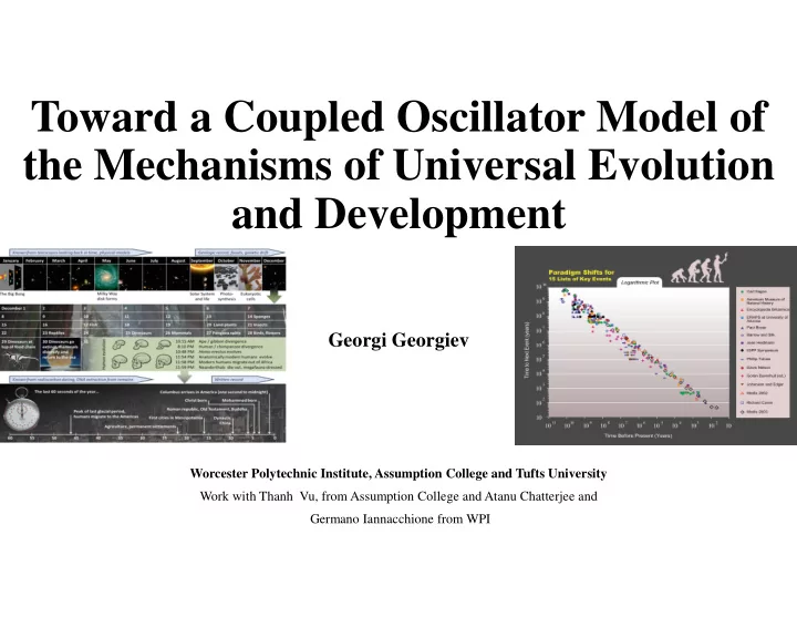
Toward a Coupled Oscillator Model of the Mechanisms of Universal Evolution and Development
Georgi Georgiev
Worcester Polytechnic Institute, Assumption College and Tufts University Work with Thanh Vu, from Assumption College and Atanu Chatterjee and Germano Iannacchione from WPI