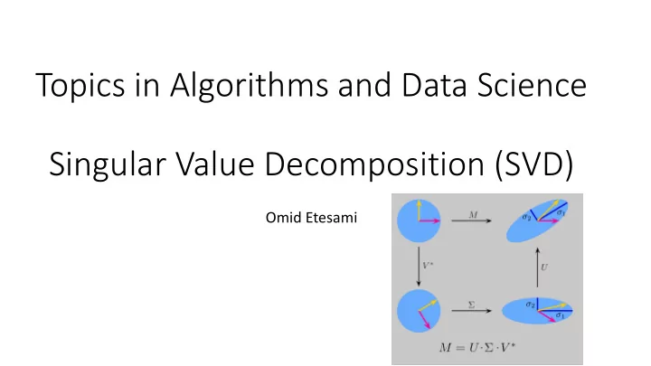
Topics in Algorithms and Data Science Singular Value Decomposition - - PowerPoint PPT Presentation

Topics in Algorithms and Data Science Singular Value Decomposition (SVD)

Omid Etesami

The problem of best-fit subpace

Best-fit subspace

n points in d-dimensional Euclidean space are given. The best-fit subspace of dimension k minimizes the sum of squared distances from the points to the subspace.

Centering data

Centering data

For the best-fit affine subspace, translate so that the center of mass of the points lies at the origin. Then find best-fit linear subspace.

Why centering works?

• Lemma. Best-fit affine subspace of dimension k for the points a1,…,an passes through

their center of mass.

Proof of lemma

• W.l.o.g. assume “center of mass = 0”.
• Let a = projection of 0 onto the affine

subspace l.

• We can write l = a + S where S is a linear

subspace.

• The sum is minimized for a = 0.

ai

The greedy approach to best subpace yields the singular vectors

The greedy approach to finding best k-dimensional subspace

S0 = {0} for i = 1 to k do Si = best-fit i-dimensional subspace among those that contain Si-1

S0 S2 S1 S3

Best-fit line

Instead of minimizing sum of squared distances we maximize sum of squared lengths of projections onto the line.

ai

1st singular vector and value

• v1 = unit vector in the direction of best-fit line
• |<ai , v1>| = length of projection of ai
• rows of n×d matrix A = data points.

1st right singular vector = v1 = argmax|v|=1 |Av| 1st singular value = |Av1|

v1

Other singular vectors

{v1,…,vi} is an orthonormal basis for Si because sum of squared lengths of projections on Si is |A vi| + sum of squared lengths of projections on Si-1. vi is the i‘th right singular vector and ơi(A) = |A vi| is the i‘th singular vector.

S0 S2 S1 S3 v1 v2

Why greedy works?

Proof by induction on k: Consider a k-dimensional subspace Tk. It has a unit vector wk orthogonal to Sk-1. Let Tk = Tk-1 + wk, such that wk is orthogonal to Tk-1.

• Sum of squared lengths of projections on Tk-1 is at most that for Sk-1.
• |A wk| ≤ |A vk|.

Sk Tk v1 w2

Singular values

We only consider non-zero singular values, i.e. i’th singular value is defined only for 1 ≤ i ≤ r = rank(A).

Lemma.

Singular Vector Decomposition

Singular Value Decomposition (SVD)

Left singular vector ui = A vi / ơi D diagonal with diagonal entries ơi U with columns ui V with columns vi

• Thm. Left singular vectors are orthogonal.

Proof:

u1 u3 u2

Uniqueness of singular values/vectors

• The sequence of singular values forms a unique non-increasing sequence.
• Singular vectors corresponding to a particular singular value ơ are any
• rthonormal basis for a unique subspace associated with ơ.

v2 v1 v’2 v’1 v’3 v3

ơ1 = ơ2 v’3 = -v3

Best rank-k approximation: Frobenius and spectral norms

Rank-k approximation

Ak is the best rank-k approximation to A under Frobenius norm.

Representing documents as vectors

I like football John likes basketball Doc 1 1 1 2 Doc 2 2 1 1 Doc 3 1 1 1

n×d term-document matrix:

Answering queries

• Each query is a d-dimensional vector x denoting the importance of

each term

• Answer = similarity (dot-product) to each document = Ax
• O(nd) time to process each query

SVD as preprocessing

When many queries, we preprocess and get We can now answer queries in O(kd + kn) time:

A u1,…,uk,v1,…,vk Ak x

preprocessing answering queries

Good when k << d, n

Spectral norm

Spectral norm of error of Ak

Spectral norm of M = ơ1

Best rank-k approximation according to spectral norm is Ak

rank-4 approximation

• f adjacency matrix

Connection of SVD with eigenvalues

Singular values and eigenvalues

• Let B = AT A.

Therefore eigenvalues of B are square of singular values of A, and eigenvectors of B are right singular vectors of A.

• If A is symmetric,

absolute value of eigenvalues of A are singular values of A, and eigenvectors of A are right singular vectors of A.

Analogue of eigenvectors and eigenvalues

• A vi = ơi ui
• AT ui = ơi vi

Computing SVD

Computing SVD by the Power Method

If ơ1 ≠ ơ2 , then Bk tends to ơ1

2k vi vi T.

Estimate of v1 = a normalized column of Bk

Inefficiency of the previous method

• Matrix multiplication takes time.
• We cannot use the potential sparsity of A.

E.g. A may be 108 × 108 but we represent it by its say 109 nonzero entries. B may have 1016 nonzero entries, so big not even possible to write.

Faster power method

Use matrix-vector multiplication instead of matrix-matrix multiplication Algorithm:

• Choose a random vector x
• Compute Bk x = AT A AT A … AT A x
• Choose Bk x normalized as v1

Component of random vector along 1st singular vector

• Lemma. Pr[ |<x, v1>| ≤ 20/d1/2] ≤ 1/10 + exp(-Ө(d)) .

Proof:

• x = y / |y| where y spherical Gaussian with unit variance
• Pr[ |<y, v1>| ≤ 1/10 ] ≤ 1/10 (<y, v1> standard normal Gaussian)
• Pr[ |y| ≥ 2 d1/2] ≤ exp(-Ө(d)) (Gaussian annulus theorem)

v1

Analysis of the power method

• Let V = span of right singular vectors with singular values ≥ (1 – Ɛ)ơ1.
• Assume |<x, v1>| ≥ δ.
• |Bk x| ≥ ơ1

2kδ.

• component of Bk x perpendicular to V ≤ [(1 – Ɛ)ơ1] 2k.

Traditional application of SVD: Principal Component Analysis

Movie recommendation

n costumers, d movies matrix A where aij= rating of user i for movie j

Principal Component Analysis (PCA)

• Assume there are k underlying factors,

e.g. “amount of comedy”, “novelty of story”, …

• each movie = k-dimensional vector
• each user = k-dimensional vector representing importance of each factor to the

user

• rating = dot-product <movie, user>
• Ak = best rank-k approximation to A yields U, V
• A – UV treated as noise

Collaborative filtering

• A has missing entries:

recommend a movie or target an ad based on previous purchases

• Assume A = small-rank matrix + noise
• One approach is to fill missing values reasonably e.g. by average rating,

then apply SVD to recover missing entries

Application of SVD: clustering mixture of spherical Gaussians

Clustering

• Partition d-dimensional points into k groups
• Finding “best” solution often NP-hard;

thus, assume stochastic models of data.

Mixture models

A class of stochastic models are mixture models, e.g. mixture of spherical Gaussians F = w1 p1 + … + wk pk

Model fitting problem

Given n i.i.d. samples drawn according to F, fit a mixture of k Gaussians to them. Possible solution:

• First, cluster the points into k clusters
• Then, fit a Gaussian to each cluster

(by choosing empirical mean and variance)

Inter-center distance

• If two Gaussian centers are very close, clustering unresolvable.
• If every two Gaussian centers are at least say six times the standard

deviation apart, clustering unambiguous.

Distance based clustering

• If x, y are independent samples from

the same Gaussian, then |x – y|2 = 2 (d1/2 ± O(1))2 σ2

• If x, y are independent samples from

two Gaussians at distance Δ, then |x – y|2 = 2 (d1/2 ± O(1))2 σ2 + Δ2 Thus, to distinguish the two cases, we need inter-center distance Δ ≥ Ω (σ d1/4).

Projection on the subspace spanned by the k centers

If we knew the subspace spanned by the k centers, we could project points on that subspace. Inter-center distances would not change, and the samples are still spherical Gaussians but now in k-space, so now a separation of Θ (σ k1/4) is enough.

How to find the subspace spanned by the k centers?

• Theorem. The best-fit subspace of dimension k

for points sampled according to the mixture distribution passes through the centers. Thus, we can find the subspace by SVD

• n a large number of sampled points.

Green points = sample points

Why best-fit subpace passes through centers?

• Best-fit line for a single Gaussian

passes through the center.

• Proof. For a unit vector x and sample point x
• Best-fit dim-k subspace for a single Gaussian

is any subspace that passes through the center.

• Proof. Greedy best-fit subspace.
• Subspace of dim k passing through k centers

is simultaneously best for all Gaussians.

Application of SVD: ranking documents and webpages

Ranking documents

Given documents in a collection, how do we rank documents according to their relevance to the collection?

• Solution. We can rank according to the length of the projection of

documents onto the first right singular vector.

I like football John likes basketball Doc 1 1 1 2 Doc 2 2 1 1 Doc 3 1 1 1

Ranking webpages

• Web as directed graph, webpages as vertices, hyperlinks as edges
• Authorities: sources of information

(with many pointers from hubs)

• Hubs: identify authorities

(with many pointers to hubs) Looks like a “circular” definition.

HITS algorithm for ranking webpages

• v = vector of authority weights
• u = vector of hub weights

Begin with a random v. Iteratively set u := Av, v := AT u. Rank authorities according to v. This is same as computing 1st singular vector through power method.

PageRank

Another ranking algorithm but based on random walks.

Application of SVD: directed Max-Cut

Directed Max-Cut problem

Given a directed graph, partition vertices into two sets S, T such that max number of edges from S to T are cut. It is NP-hard. Equivalently, we want to find 0-1 vector x such that xT A (1-x) is maximized.

Dark edges are cut

Approximation algorithm

For constant k, maximize xT Ak (1-x) instead of xT A (1-x).

rank-4 approximation

• f adjacency matrix

Why the objective function doesn’t change much?

rank-4 approximation

• f adjacency matrix

Optimizing the objective function for low rank matrices?

This is NP-hard even for k = 1. (Reduction from Set Partition problem) We approximate instead.

Rounding the singular vectors

Optimizing the objective function for rounded vectors