
SLIDE 1
CSE 461 University of Washington 1
Topic
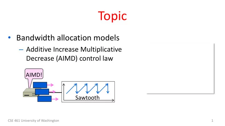
- Bandwidth allocation models
– Additive Increase Multiplicative Decrease (AIMD) control law
AIMD! Sawtooth
Topic Bandwidth allocation models Additive Increase Multiplicative - - PowerPoint PPT Presentation
Topic Bandwidth allocation models Additive Increase Multiplicative Decrease (AIMD) control law AIMD! Sawtooth CSE 461 University of Washington 1 Recall Want to allocate capacity to senders Network layer provides feedback
CSE 461 University of Washington 1
AIMD! Sawtooth
CSE 461 University of Washington 2
– Network layer provides feedback – Transport layer adjusts offered load – A good allocation is efficient and fair
– Several different possibilities …
CSE 461 University of Washington 3
CSE 461 University of Washington 4
CSE 461 University of Washington 5
CSE 461 University of Washington 6
Rest of Network Bottleneck Router Host 1 Host 2 1 1 1
CSE 461 University of Washington 7
Host 1 Host 2
1 1
Fair Efficient Optimal Allocation Congested
CSE 461 University of Washington 8
Host 1 Host 2
1 1
Fair, y=x Efficient, x+y=1 Optimal Allocation Congested Multiplicative Decrease Additive Increase
CSE 461 University of Washington 9
Host 1 Host 2
1 1
Fair Efficient Congested A starting point
CSE 461 University of Washington 10
Host 1 Host 2
1 1
Fair Efficient Congested A starting point
CSE 461 University of Washington 11
Multiplicative Decrease Additive Increase Time Host 1 or 2’s Rate
CSE 461 University of Washington 12
CSE 461 University of Washington 13
Signal Example Protocol Pros / Cons Packet loss TCP NewReno Cubic TCP (Linux) Hard to get wrong Hear about congestion late Packet delay Compound TCP (Windows) Hear about congestion early Need to infer congestion Router indication TCPs with Explicit Congestion Notification Hear about congestion early Require router support
CSE 461 University of Washington 14
What’s up? Internet
CSE 461 University of Washington 15
CSE 461 University of Washington 16
Congestion collapse
CSE 461 University of Washington 17
CSE 461 University of Washington 18
CSE 461 University of Washington 19
CSE 461 University of Washington 20
1988 1990 1970 1980 1975 1985 Origins of “TCP” (Cerf & Kahn, ’74) 3-way handshake (Tomlinson, ‘75) TCP Reno (Jacobson, ‘90) Congestion collapse Observed, ‘86 TCP/IP “flag day” (BSD Unix 4.2, ‘83) TCP Tahoe (Jacobson, ’88)
Pre-history Congestion control
. . . TCP and IP (RFC 791/793, ‘81)
CSE 461 University of Washington 21
Tick Tock!
CSE 461 University of Washington 22
Ack 1 2 3 4 5 6 7 8 9 10 20 19 18 17 16 15 14 13 12 11 Data
CSE 461 University of Washington 23
Fast link Fast link Slow (bottleneck) link Queue
CSE 461 University of Washington 24
Fast link Fast link Slow (bottleneck) link Segments “spread out”
CSE 461 University of Washington 25
Slow link Acks maintain spread
CSE 461 University of Washington 26
Slow link Segments spread Queue no longer builds
CSE 461 University of Washington 27
CSE 461 University of Washington 28
CSE 461 University of Washington 29
Slow-start
CSE 461 University of Washington 30
CSE 461 University of Washington 31
CSE 461 University of Washington 32
AI Fixed Time Window (cwnd) Slow-start
CSE 461 University of Washington 33
CSE 461 University of Washington 34
AI Fixed Time Window ssthresh cwndC cwndIDEAL AI phase Slow-start
CSE 461 University of Washington 35
Increment cwnd by 1 packet for each ACK
CSE 461 University of Washington 36
Increment cwnd by 1 packet every cwnd ACKs (or 1 RTT)
CSE 461 University of Washington 37
– Start with cwnd = 1 (or small value) – cwnd += 1 packet per ACK
– cwnd += 1/cwnd packets per ACK – Roughly adds 1 packet per RTT
– Switch to AI when cwnd > ssthresh – Set ssthresh = cwnd/2 after loss – Begin with slow-start after timeout
CSE 461 University of Washington 38
CSE 461 University of Washington 39
AIMD sawtooth
CSE 461 University of Washington 40
ACK clock, followed by Additive Increase
CSE 461 University of Washington 41
CSE 461 University of Washington 42
Ack 1 2 3 4 5 5 5 5 5 5
CSE 461 University of Washington 43
Ack 10 Ack 11 Ack 12 Ack 13
. . .
Ack 13 Ack 13 Ack 13 Data 14
. . .
Ack 13 Ack 20
. . . . . .
Data 20
Third duplicate ACK, so send 14 Retransmission fills in the hole at 14 ACK jumps after loss is repaired . . . . . . Data 14 was lost earlier, but got 15 to 20
CSE 461 University of Washington 44
CSE 461 University of Washington 45
CSE 461 University of Washington 46
Ack 1 2 3 4 5 5 5 5 5 5
CSE 461 University of Washington 47
Ack 12 Ack 13 Ack 13 Ack 13 Ack 13 Data 14 Ack 13 Ack 20
. . . . . .
Data 20
Third duplicate ACK, so send 14 Data 14 was lost earlier, but got 15 to 20 Retransmission fills in the hole at 14 Set ssthresh, cwnd = cwnd/2
Data 21 Data 22
More ACKs advance window; may send segments before jump
Ack 13
Exit Fast Recovery
CSE 461 University of Washington 48
CSE 461 University of Washington 49
MD of ½ , no slow-start ACK clock running TCP sawtooth
CSE 461 University of Washington 50
CSE 461 University of Washington 51
!!
CSE 461 University of Washington 52
CSE 461 University of Washington 53
Signal Example Protocol Pros / Cons Packet loss Classic TCP Cubic TCP (Linux) Hard to get wrong Hear about congestion late Packet delay Compound TCP (Windows) Hear about congestion early Need to infer congestion Router indication TCPs with Explicit Congestion Notification Hear about congestion early Require router support
CSE 461 University of Washington 54
CSE 461 University of Washington 55
CSE 461 University of Washington 56