time vs frequency resolution
play

Time vs. frequency resolution Each coefficient of a Fourier spectra - PowerPoint PPT Presentation

Time vs. frequency resolution Each coefficient of a Fourier spectra of a signal (image) provides Image Analysis information about the signal contents of that frequency. Wavelets and Multiresolution Processing However, the Fourier coefficients


  1. Time vs. frequency resolution Each coefficient of a Fourier spectra of a signal (image) provides Image Analysis information about the signal contents of that frequency. Wavelets and Multiresolution Processing However, the Fourier coefficients contain no spatial knowledge . On the other hand, each spatial coefficient, i.e. sample, contains no frequency information . Niclas Börlin niclas.borlin@cs.umu.se In image analysis, different frequencies correspond to objects of different sizes . Department of Computing Science Umeå University Low frequencies correspond to slow changes over a large area . High frequencies correspond to fast changes over a small area . February 20, 2009 Wavelets allow us to analyse a combination of spatial and frequency information. Niclas Börlin (CS, UmU) Wavelets and Multiresolution Processing February 20, 2009 1 / 24 Niclas Börlin (CS, UmU) Wavelets and Multiresolution Processing February 20, 2009 2 / 24 The Fourier vs. Wavelet transformation The Image Pyramid A closely related concept is the Image pyramid . Images of different spatial resolutions, form levels of the pyramid. The Fourier transform uses sinusoids of infinite duration as basis functions. Wavelet transforms uses small waves (wavelets) of limited duration as basis functions. The Fourier transform gives information about images frequency decomposition. The Wavelet transforms have resolution in the frequency domain The original image with the highest resolution is at level J , the as well as in the spatial domain (what frequencies are in the lowest pyramid level. image — and where ). Each higher level contain a lower resolution image, usually half. Wavelets are conceptually similar to musical scores: The image at the top Level 0 contain only one pixel. ◮ Which tones, and The total number of pixels in a P + 1 level pyramid is ◮ when to play them? � 1 1 1 � ≤ 4 N 2 3 N 2 . 1 + ( 4 ) 1 + ( 4 ) 2 + · · · + ( 4 ) P Niclas Börlin (CS, UmU) Wavelets and Multiresolution Processing February 20, 2009 3 / 24
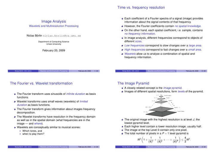
 Niclas Börlin (CS, UmU) Wavelets and Multiresolution Processing February 20, 2009 4 / 24

  2. The Approximation and Prediction Residual Pyramids The Approximation and Prediction Residual Pyramids Level j of the Approximation Pyramid is formed by smoothing and downsampling the image at level j + 1. Level j of the Prediction Residual Pyramid is formed as the difference between the upsampled and interpolated level j − 1 image, and the level j approximation image. Niclas Börlin (CS, UmU) Wavelets and Multiresolution Processing February 20, 2009 5 / 24 Niclas Börlin (CS, UmU) Wavelets and Multiresolution Processing February 20, 2009 6 / 24 Subband coding and filter banks Perfect reconstruction The concept of subband coding is to split a signal into two (or The lowpass filter h 0 ( n ) produce the approximation subband more) components that completely describes the input. f lp ( n ) . This is performed in conjunction with two filter banks . The highpass filter h 1 ( n ) produce the detail subband f hp ( n ) . The analysis filter bank uses filters h 0 ( n ) and h 1 ( n ) to split the If the filter banks are chosen properly, the signal can be perfectly input sequence f ( n ) into two half-length sequences ( subbands ) reconstructed from its subbands f lp ( n ) and f hp ( n ) . f lp ( n ) and f hp ( n ) . The synthesis filter bank g 0 ( n ) and g 1 ( n ) combines f lp ( n ) and f hp ( n ) to form the reconstructed signal ˆ f ( n ) . If the analysis filter bank is recursively applied to the approximation subband, we obtain an approximation pyramid. Niclas Börlin (CS, UmU) Wavelets and Multiresolution Processing February 20, 2009 7 / 24 Niclas Börlin (CS, UmU) Wavelets and Multiresolution Processing February 20, 2009 8 / 24

  3. 2D subbands 2D subband example Subband coding for a 2D signal is separable and may be applied sequentially along the rows and columns. Furthermore, the downsampling can be applied once after each analysis stage, significantly improving performance. The result is four subbands: The approximation a ( m , n ) , the vertical detail d V ( m , n ) , the horizontal detail d H ( m , n ) , and the diagonal detail d D ( m , n ) . Niclas Börlin (CS, UmU) Wavelets and Multiresolution Processing February 20, 2009 9 / 24 Niclas Börlin (CS, UmU) Wavelets and Multiresolution Processing February 20, 2009 10 / 24 Multiresolution analysis The Haar Transform The Haar transform basis functions are the oldest and simplest Multiresolution analysis (MRA) uses a scaling function ϕ ( x ) to known orthonormal wavelets. create a series of approximations of a signal or image, each The Haar transform is separable and expressible in matrix form differing by a factor of 2 from its nearest neighboring approximation. T = HFH T , Wavelet functions ψ ( x ) are then used to encode the difference ( detail ) in information between adjacent approximations. where F is an N × N image, H is an N × N transformation matrix that contains the Haar basis functions, and T is the resulting MRA defines a set of requirements for the scaling functions. N × N transform. Given a scaling function that meets these requirements we The basis functions are scaled and translated versions of a define a wavelet function to use. mother wavelet . Niclas Börlin (CS, UmU) Wavelets and Multiresolution Processing February 20, 2009 11 / 24 Niclas Börlin (CS, UmU) Wavelets and Multiresolution Processing February 20, 2009 12 / 24

  4. The Haar Transform The Haar scaling and wavelet functions Assume N = 2 n , 0 ≤ p ≤ n − 1, k = 2 p + q − 1, and The Haar transform correspond to the Haar scaling function � 0 or 1 , p = 0 � 1 0 ≤ x < 1 q = p � = 0 . ϕ ( x ) = 1 ≤ q ≤ 2 p , 0 otherwise and the Haar wavelet function Then the Haar basis functions h k ( z ) are defined as  1 0 ≤ x < 0 . 5 1  h 0 ( z ) = h 00 ( z ) = , z ∈ [ 0 , 1 ] , and √ − 1 0 . 5 ≤ x < 1 ψ ( x ) = . N 0 otherwise  ( q − 1 ) / 2 p ≤ z < ( q − 0 . 5 ) / 2 p , 2 p / 2  The shifted and scaled versions of the Haar functions are defined as 1  ( q − 0 . 5 ) / 2 p ≤ << q / 2 p , − 2 p / 2 h k ( z ) = h pq ( z ) = √ ϕ j , k ( x ) = 2 j / 2 ϕ ( 2 j x − k ) , N 0 otherwise, z ∈ [ 0 , 1 ] .  ψ j , k ( x ) = 2 j / 2 ψ ( 2 j x − k ) , We get where k determines the position of the functions and j determines the  1 1 1 1  width. 1 � 1 � 1 1 1 − 1 − 1 1 The value of j corresponds to the layer in the image pyramid.  √ √  H 2 = √ and H 4 = √   1 − 1 2 2 0 0 − 2 4 The wavelet function ψ ( x ) corresponds to the difference between layer  √ √  0 0 2 − 2 j and j + 1. Niclas Börlin (CS, UmU) Wavelets and Multiresolution Processing February 20, 2009 13 / 24 Niclas Börlin (CS, UmU) Wavelets and Multiresolution Processing February 20, 2009 14 / 24 The Haar scaling and wavelet functions The Discrete 1D wavelet transform 1 � W ϕ ( j 0 , k ) = √ f ( x ) ϕ j 0 , k ( x ) M x 1 � W ψ ( j , k ) = f ( x ) ψ j , k ( x ) √ M x ∞ 1 1 � � � f ( x ) = √ W ϕ ( j 0 , k ) ϕ j 0 , k ( x ) + √ W ψ ( j , k ) ψ j , k ( x ) , M M k j = j 0 k where j 0 = 0, M = 2 J , x = 0 , 1 , . . . , M − 1, j = 0 , 1 , . . . , J − 1, k = 0 , 1 , . . . , 2 j − 1. The functions ϕ ( x ) and ψ ( x ) are assumed to form an orthonormal base (or tight frame). Niclas Börlin (CS, UmU) Wavelets and Multiresolution Processing February 20, 2009 15 / 24 Niclas Börlin (CS, UmU) Wavelets and Multiresolution Processing February 20, 2009 16 / 24

  5. Time-frequency resolution The Discrete 2D wavelet transform Each tile represent an equal portion of the time-frequency plane. There is a trade-off between the resolution in time and frequency. Higher resolution in frequency (low frequencies) ⇔ lower resolution in time. Higher resolution in time (high frequencies) ⇔ lower resolution in frequency. Niclas Börlin (CS, UmU) Wavelets and Multiresolution Processing February 20, 2009 17 / 24 Niclas Börlin (CS, UmU) Wavelets and Multiresolution Processing February 20, 2009 18 / 24 The Fast Wavelet Transform (FWT) 2D discrete wavelet transform using Haar basis The Fast Wavelet Transform (FWT) is essentially a recursive interleaving application of the smoothing ( ϕ ( x ) ) and differencing ( ψ ( x ) ) filters and the downsampling. The first application corresponds to the highest frequencies (narrowest wavelets). Each successive downsampling corresponds to widening of the wavelet by a factor of two. Niclas Börlin (CS, UmU) Wavelets and Multiresolution Processing February 20, 2009 19 / 24 Niclas Börlin (CS, UmU) Wavelets and Multiresolution Processing February 20, 2009 20 / 24

  6. Multiscale DWT Wavelet edge detection Niclas Börlin (CS, UmU) Wavelets and Multiresolution Processing February 20, 2009 21 / 24 Niclas Börlin (CS, UmU) Wavelets and Multiresolution Processing February 20, 2009 22 / 24 Wavelet noise removal Other wavelets The optimal wavelet function is called Daubechies and have self-similar, i.e. fractal, characteristics. Niclas Börlin (CS, UmU) Wavelets and Multiresolution Processing February 20, 2009 23 / 24 Niclas Börlin (CS, UmU) Wavelets and Multiresolution Processing February 20, 2009 24 / 24

Download Presentation
Download Policy: The content available on the website is offered to you 'AS IS' for your personal information and use only. It cannot be commercialized, licensed, or distributed on other websites without prior consent from the author. To download a presentation, simply click this link. If you encounter any difficulties during the download process, it's possible that the publisher has removed the file from their server.

Recommend


More recommend