Three-Dimensional Biomechanical Analysis of Human Movement Motion - PowerPoint PPT Presentation

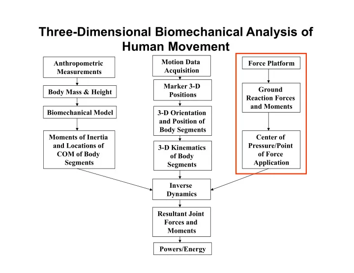
Three-Dimensional Biomechanical Analysis of Human Movement Motion Data Anthropometric Force Platform Acquisition Measurements Marker 3-D Ground Body Mass & Height Positions Reaction Forces and Moments Biomechanical Model 3-D Orientation and Position of Body Segments Moments of Inertia Center of and Locations of Pressure/Point 3-D Kinematics COM of Body of Force of Body Segments Application Segments Inverse Dynamics Resultant Joint Forces and Moments Powers/Energy

Ground Reaction Forces § Vertical Force § A/P Force Horizontal Shear § M/L Force § Twisting Torque (free moment) F=F x +F y +F z F z F y F x

Ground Reaction Forces

Force Platforms Piezoelectric type A piezoelectric material, quartz crystal, will generate an electric charge when subject to mechanical strain. Quartz crystals are cut into disks that respond to mechanical strain in a single direction. Strain Gauge type Use strain gauge to measure stress in machined aluminum transducers (load cells). Deformation of the material causes a change in the resistance and thus a change in the voltage (Ohms Law: V = I * R).

Two Common Types of Force Plates A flat plate supported A flat plate supported by four triaxial by one centrally transducers instrumented pillar

AMTI (Strain Gauge) Force Platform Output signals from the platform: F x : the anterior/posterior force F y : the medial/lateral force F z : the vertical force M x : the moment about the anterior/posterior axis M y : the moment about the medial/lateral axis M z : the moment about the vertical axis

Kistler (Strain Gauge) Force Platform

Center of Pressure (COP) F T z Center of Pressure All the forces acting between the foot and the ground can be summed and yield a single reaction force vector (F) and a twisting torque vector (T z about the vertical axis). Under normal condition there is no physical way to apply T x and T y . The point of application of the ground reaction force on the plate is the center of pressure (COP).

Computation of the COP Z F Generally, the true T z origin of the plate is not at the geometric center of COP (x, y, 0) X r the plate surface. The manufacturer usually provides the offset data. Y true origin (a, b, c) The moment measured from the plate is equal to the moment caused by F about the true origin plus T z .

Computation of the COP Z F T z COP (x, y, 0) X r Y true origin (a, b, c) M = r × F + T z

Computation of the COP M = r × F + T z r = (x-a, y-b, -c) known: a, b, c; unknown: x, y F = (F x , F y , F z ) force values from plate outputs T z = (0, 0, T z ) unknown: T z M = (M x , M y , M z ) torque values from plate outputs

T z COP (a x , a y , a z ) r cop r cop = [ a x , a y , a z ] M GRF = r cop × F + T z

Computation of the COP M x = (y-b) F z + c F y M y = -c F x - (x-a) F z Z Z Z F F F Tz Tz Tz M z = (x-a) F y - (y-b) F x + T z COP (x, y, 0) COP (x, y, 0) COP (x, y, 0) x = -(M y + cF x )/F z +a X X X r r r y = (M x - cF y )/F z +b T z = M z - (x-a)F y + (y-b)F x Y Y Y true origin (a, b, c) true origin (a, b, c) true origin (a, b, c) M = r × F + Tz M = r × F + Tz

Force Plate Coordinate System Y f O FP X f r FPCS COP r OFP in GCS Z f r cop Z g r cop = R r FPCS + r OFP X g Y g known information during laboratory setup (calibration)

GRF in Global Coordinate System Y f GRF Tz O FP X f Z f Z g GRF GCS = R GRF FPCS X g Tz GCS = R Tz FPCS Y g

Three-Dimensional Biomechanical Analysis of Human Movement Motion Data Anthropometric Force Platform Acquisition Measurements Marker 3-D Ground Body Mass & Height Positions Reaction Forces and Moments Biomechanical Model 3-D Orientation and Position of Body Segments Moments of Inertia Center of and Locations of Pressure/Point 3-D Kinematics COM of Body of Force of Body Segments Application Segments Inverse Dynamics Resultant Joint Forces and Moments Powers/Energy

Determining Body Segment and Joint Kinematics Three-step procedure § Three-dimensional marker positions § Body segment (limb) positions and orientations (assuming rigid body) § Relative orientation and movement of limb segments (joint kinematics)

Step #1 … Marker Position • 3-D reconstruction from several 2-D images – Each point seen by at least 2 cameras • Vicon system displays reconstructed points (saves you a ton of time) • Now, for Step #2

Step #2 … Segment positions and orientations • Defining segment coordinate systems – Position described by the segment origin – Orientation provides the “ absolute ” angles

Segment definitions (the need for marker sets) • Absolutely necessary for kinematic variables to be measured/calculated Key definitions in 2D and 3D kinematics: • Segment endpoints for creation of links • Segment dimensions (body segment parameters) • Orientation of segments, for angular data

Pelvis marker set (general)

Helen Hayes marker set

Foot marker set (general)

Step #3 … Relative position and orientations between segments Relationship between the Local c.s. (LCS) and the Global c.s. (GCS) x i y i z i § Linear z § Rotational x y

Linear Kinematics of a Rigid Body Position Vector: A vector starting from the origin of a coordinate system to a point in the space is defined as the position vector of that point. Y P • r Q/P r P Q r Q • X O Displacement Vector: The vector difference of two position vectors is defined as the displacement vector from the first point (P) to the second point (Q). r Q/P = r Q - r P

Linear Transformation Assume that GCS (x,y,z) and LCS (x i ,y i ,z i ) coincide z i o i with each other in the y i beginning (t = 0). r pi x i z i The LCS is only translating, o i y i that is there is no rotational p r oi movement. x i z At time t, the LCS moves to a location which is r p represented by a position vector of r oi . o y x r p = r pi + r oi

Rotational Transformation z Assume that GCS (x,y,z) and LCS (x i ,y i ,z i ) coincide p with each other in the z i beginning (t = 0). r pi y i y At time t, the LCS rotates x i with respect to the GCS and z reaches a final orientation. x p r p = R r pi z i y i r p R : rotation matrix from LCS to GCS x i x

Rotational Matrix r p = R r pi z If directions of the x i , y i , and p z i of the LCS axes can be z i r p y i expressed by unit vectors v 1 , v 2 , and v 3 , respectively, in the GCS, the rotation matrix from the LCS to GCS x i x is defined as R v i v i v i v v v • • • & # & # 1 2 3 1x 2x 3x $ ! $ ! R v j v j v j v v v = • • • = 1 2 3 1y 2y 3y $ ! $ ! v k v k v k v v v $ • • • ! $ ! % " % " 1 2 3 1z 2z 3z

Relationship between the LCS and Fixed (Global) coordinate system (GCS) Linear transformation+Rotational transformation o i x i y i r pi r p = R r pi + r oi z i p z r oi r p x y

Relationship between the LCS and Fixed (Global) coordinate system (GCS) 4 × 4 Transformation Matrix r a a a r r & # & # & # & # px 11 12 13 pxi oix $ ! $ ! r p = R r pi + r oi $ ! $ ! r a a a r r = + $ ! $ ! py 21 22 23 pyi oiy $ ! $ ! r a a a r r $ ! $ ! $ ! $ ! % " % " % " % " pz 31 32 33 pzi oiz r a a a r r & # & # & # px 11 12 13 oix pxi $ ! $ ! $ ! r a a a r r py 21 22 23 oiy pyi $ ! $ ! $ ! = r a a a r r $ ! $ ! $ ! pz 31 32 33 oiz pzi $ ! $ ! $ ! 1 0 0 0 1 1 % " % " % "

Determining Joint Kinematics If the orientation of two local coordinate systems (two adjacent body segments) are known, then the relative orientation between these two segments can be determined. y j z j z i o j y i P r p = R i r pi (1) x j o i z r p = R j r pj (2) r pj r pi (1)=(2) x i r p R i r pi = R j r pj r pi = R i -1 R j r pj o y x

Determining Joint Angles 3-D joint angles are concerned about the relative orientation between any two adjacent body segments, therefore, only the rotation matrix is needed for computation. r pi = R i -1 R j r pj =R i/j r pj

Basic Rotational Matrices Rotation about the X-axis z z i y i θ r p = R r pi θ x i y x $ ' 1 0 0 & ) R = 0 cos θ − sin θ & ) & ) 0 sin θ cos θ % (

Basic Rotational Matrices Rotation about the Y-axis z z i φ r p = R r pi y i x i y φ x $ ' cos φ 0 sin φ & ) R = 0 1 0 & ) & ) − sin φ 0 cos φ % (

Basic Rotational Matrices Rotation about the Z-axis z z i y i r p = R r pi γ y γ x i x $ ' cos γ − sin γ 0 & ) R = sin γ cos γ 0 & ) & ) 0 0 1 % (

Cardan / Euler Angles Cardan/Euler angles are defined as a set of three finite rotations assumes to take place in sequence to achieve the final orientation (x 3 ,y 3 ,z 3 ) from a reference frame (x 0 ,y 0 ,z 0 ). Cardan angles: all three axes are different Euler angles: the 1 st and last axes are the same z 0 y 2 y 2 z 2 z 2 z 1 z 1 y 1 z 3 y 3 θ 2 y 1 θ 3 y 0 x 0 x 1 θ 1 x 1 x 3 x 2 x 2