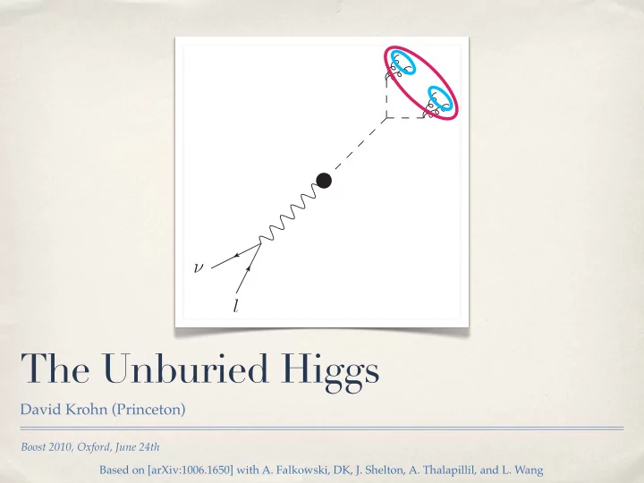
The Unburied Higgs David Krohn (Princeton) Boost 2010, Oxford, June - - PowerPoint PPT Presentation

Boost 2010, Oxford, June 24th

The Unburied Higgs

David Krohn (Princeton)

Based on [arXiv:1006.1650] with A. Falkowski, DK, J. Shelton, A. Thalapillil, and L. Wang

l ν

Outline

✤ The Buried Higgs Model ✤ Challenging Phenomenology ✤ Discovering this with Substructure ✤ Conclusions

Takeaway

✤ Use jet substructure to find Higgs decaying to four gluons ✤ New observables sensitive to color flow ✤ Potential application to more general BSM physics (hidden valley..)

Buried Higgs

✤ Model designed to realize interesting signatures ✤ Details not important to us. For concreteness though: ✤ Start with SUSY little-Higgs model with SU(3)->SU(2) ✤ Higgs is a PGB. Also have extra Goldstone: the singlet a ✤ a is naturally a few GeV, couples to the Higgs

• Buried Higgs, B. Bellazzini, C. Csaki, A. Falkowski, A. Weiler, [arXiv:0906.3026] Phys.Rev. D80 (2009) 075008
• Charming Higgs, B. Bellazzini, C. Csaki, A. Falkowski, A. Weiler, [arXiv:0910.3210] Phys.Rev. D81 (2010) 075017

Lha2 ∼ v f 2 h(∂µa)2

Buried Higgs Phenomenology

✤ The process h->aa can dominate the Higgs

decay

✤ a will decay to gluons via a loop ✤ Thus the main decay mode of the Higgs

can be (depending on the a mass)

✤ h->aa->gggg

bb gg ΓΓ ΤΤ cc

2 4 6 8 10 109 107 105 0.001 0.1 mΗGeV BR

Goal

✤ This Higgs is difficult to discover in colliders because it essentially

decays into dijets

✤ Thus it is ``buried’’ ✤ However, the jets exhibit some non-QCD like behavior. ✤ This might be a sufficient handle to allow us to ``unbury’’ the

model

Substructure with a SM Higgs

✤ How do we look for the SM Higgs using substructure? ✤ In V+h channel: ✤ Look for jet recoiling against W/Z ✤ Groom the jet to improve mass resolution ✤ Require two b-tags

• Jet substructure as a new Higgs search channel at the LHC, J. M. Butterworth, A. R. Davison, M. Rubin, G. P. Salam,

[arXiv:0802.2470] Phys.Rev.Lett. 100 (2008) 242001

• Fat Jets for a Light Higgs, T. Plehn, G. P. Salam, M. Spannowsky, [arXiv:0910.5472] Phys.Rev.Lett. 104 (2010) 111801

✤ For the Buried Higgs there is no b-jet. ✤ Need to compensate for this. ✤ However, a boosted Buried Higgs is

distinguished in (at least) three ways

• 1. Each a subjet has a relatively low mass

(ma<2mb)

• 2. Each subjet inside the Higgs has

roughly the same mass

• 3. Color is only resolved at the very end of

the decay, at low mass and small angles.

l ν

Observables

✤ Therefore we define three substructure observables sensitive to these

characteristics

• 1. A subjet mass cut
• 2. A mass democracy variable
• 3. A color flow variable

m ≡ m(j1) + m(j2) 2 < 10 GeV, α = min m(j1) m(j2), m(j2) m(j1)

• β =

pT (j3) pT (j1) + pT (j2),

Grooming Procedure

✤ To improve our mass resolution we apply jet

trimming to our fat jets

✤ Although reconstructing boosted heavy

particles was not the original goal of Jet Trimming, we find it can be quite effective.

✤ In limited testing can be competitive with

filtering/pruning (see Soper and Spannowsky).

• Jet Trimming, DK, J. Thaler, L. Wang, [arXiv:0912.1342] JHEP 1002 (2010) 084
• Combining subjet algorithms to enhance ZH detection at the LHC, D. E. Soper, M. Spannowsky, [arXiv:1005.0417]

Mass [GeV]

400 420 440 460 480 500 520 540 560 580 600

Cross Section [A.U.]

0.05 0.1 0.15 0.2 0.25

T

anti-k trimmed

T

anti-k

✤ Important point: filtering/pruning/trimming remove

the soft radiation essential to our color flow

• bservables

✤ Must use trimmed jet for mass cut, untrimmed jet for

substructure analysis!

Results

Results (W+h)

• σsig (fb)

σbg (fb) S/B S/ √ B pT (j) > 200 GeV 16 30000 0.00052 0.9 subjet mass 12 19000 0.00062 0.9 Higgs window 7.1 400 0.018 3.6 α > 0.7 4.1 140 0.030 3.5 β < 0.005, pmin

T

= 1 GeV 0.67 0.74 0.90 7.8 β < 0.005, pmin

T

= 5 GeV 2.9 2.6 0.11 5.7

L=100 fb-1

Mass democracy Color flow Low subjet masses

Results (tt+h)

L=100 fb-1

σsig (fb) σbg (fb) S/B S/ √ B preselection 8.1 6700 0.001 1.0 pT (j) > 125 GeV 3.1 750 0.004 1.1 pT (j2) > 40 GeV, m < 10 GeV 0.58 22 0.03 1.2 m(j) = mh ± 10 GeV 0.45 3.9 0.1 2.3 α > 0.7 0.40 2.0 0.2 2.9 β < 0.03, pmin

T

= 1 GeV 0.28 0.21 1.3 6.1 β < 0.03, pmin

T

= 5 GeV 0.29 0.25 1.1 5.7

✤ Note that here you’re helped by the fact that there are no

combinatoric ambiguities

✤ Every b comes from a top

0.05 0.1 0.15 0.2 0.25 0.3 0.35 0.4 0.45 60 70 80 90 100 110 120 130 140

Cross Section [fb/10-GeV] Mass [GeV]

Signal Background 0.5 1 1.5 2 2.5 60 70 80 90 100 110 120 130 140

Cross Section [fb/10-GeV] Mass [GeV]

Signal Background

W+h Higgs mass tt+h Higgs mass

mh = 80 GeV mh = 100 GeV mh = 120 GeV pp → hW S/ √ B 6.6 (4.8) 7.8 (5.7) 7.0 (6.9) S/B 0.34 (0.067) 0.90 (0.11) 0.80 (0.24) pp → ht¯ t S/ √ B 6.1 (5.9) 6.1 (5.7) 7.1 (7.1) S/B 1.1 (0.97) 1.3 (1.1) 2.5 (2.5)

L=100 fb-1

Another Approach (Chen et. al.)

• Search for the Elusive Higgs Boson Using Jet Structure at LHC, C. Chen, M. Nojiri, W. Sreethawong, [arXiv:1006.1151]

200

mjj (GeV)

5 10 15 20 25 20 40 60 80 100 120 140 160 180 200

Jet algorithm σS (fb) S/ √ B CA 0.43 3.75 KT 0.53 5.06

✤ Look in different kinematic regime ✤ Each a gets its own jet (R=0.5) ✤ Require each subjet show a mass drop ✤ Require symmetric subjets ✤ Cut on jet mass

Note that this is for L = 30 fb−1

Conclusions

✤ Substructure techniques help us to ``unbury’’ h->aa->gggg ✤ Pushing detector technology (resolutions/thresholds) can lead to

immediate and significant improvements in this sort of analysis.

✤ Allows one to push harder with color flow cuts ✤ Color sensitive substructure observables may find wider application

in BSM analyses.