The Theory of Statistical Comparison with Applications in Quantum - PowerPoint PPT Presentation

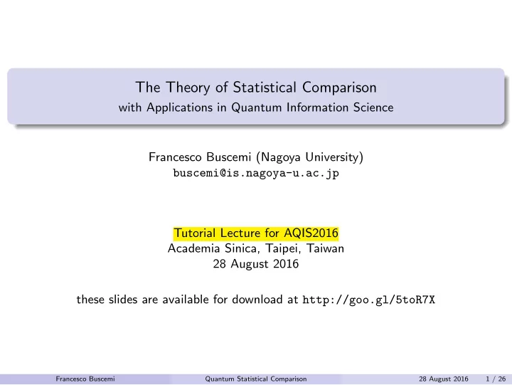
The Theory of Statistical Comparison with Applications in Quantum Information Science Francesco Buscemi (Nagoya University) buscemi@is.nagoya-u.ac.jp Tutorial Lecture for AQIS2016 Academia Sinica, Taipei, Taiwan 28 August 2016 these slides are available for download at http://goo.gl/5toR7X Francesco Buscemi Quantum Statistical Comparison 28 August 2016 1 / 26

Prerequisites Prerequisites for the first part (general results): ✔ basics of probability and information theory: random variables, joint and conditional probabilities, expectation values, etc ✔ in particular, noisy channels as probabilistic maps between two sets w : A → B : given input a ∈ A , the probability to have output b ∈ B is given by conditional probability w ( b | a ) ✔ basics of quantum information theory: Hilbert spaces, density operators, ensembles, POVMs, quantum channels ≡ CPTP maps, composite systems and tensor products, etc Prerequisites for the second part (applications): ✔ resource theories, in particular, quantum thermodynamics: idea of the general setting and of the problem treated (in particular, some knowledge of majorization theory is helpful) ✔ entanglement and quantum nonlocality: general ideas such as Bell inequalities, nonocal games, entangled states, etc ✔ open systems dynamics: basic ideas such as reduced dynamics, Markov chains and Markovian evolutions, divisibility, etc (quantum case only sketched, see references) Francesco Buscemi Quantum Statistical Comparison 28 August 2016 2 / 26

Part I Statistical Comparison: General Results Francesco Buscemi Quantum Statistical Comparison 28 August 2016 3 / 26

Statistical Games ( aka Decision Problems) ✔ Definition. A statistical game is a triple (Θ , U , ℓ ) , where Θ = { θ } and U = { u } are finite sets, and ℓ is a function ℓ ( θ, u ) ∈ R . ✔ Interpretation. We assume that θ is the value of a parameter influencing what we observe, but that cannot be observed “directly.” Now imagine that we have to choose an action u , and that this choice will earn or cost us ℓ ( θ, u ) . For example, θ is a possible medical condition, u is the choice of treatment, and ℓ ( θ, u ) is the overall “efficacy.” ✔ Resource. Before choosing our action, we are allowed “to spy” on θ by performing an experiment (i.e., visiting the patient). Mathematically, an experiment is given as a sample set X = { x } (i.e., observable symptoms) together with a conditional probability w ( x | θ ) or, equivalently, a family of distributions { w θ ( x ) } θ ∈ Θ . ✔ Probabilistic decision. The choice of an action can be probabilistic (i.e., patients with the same symptoms are randomly given different therapies). Hence, a decision is mathematically given as a conditional probability d ( u | x ) . experiment decision Θ − → X − → U � � � = ⇒ ℓ ( θ, u ) θ − → x − → u w ( x | θ ) d ( u | x ) ✔ Example in information theory. Imagine that θ is the input to a noisy channel, x is the output we receive, and u is the message we decode. Francesco Buscemi Quantum Statistical Comparison 28 August 2016 4 / 26

How much is an experiment worth? experiment decision Θ − → X − → U � � � = ⇒ ℓ ( θ, u ) − → − → θ x u w ( x | θ ) d ( u | x ) ✔ experiments help us choosing the action “sensibly.” How much would you pay for an experiment? ✔ Expected payoff. E ℓ [ w ] � max d ( u | x ) u,x,θ ℓ ( θ, u ) d ( u | x ) w ( x | θ ) 1 � | Θ | . (Bayesian assumption for simplicity, but this is not necessary.) ✔ consider now a different experiment (but about the same unknown parameter θ ) with sample set Y = { y } and conditional probability w ′ ( y | θ ) . Which is better between w ( x | θ ) and w ′ ( y | θ ) ? ✔ such questions are considered in the theory of statistical comparison: a very deep field of mathematical statistics, pioneered by Blackwell and greatly developed by Le Cam and Torgersen, among others. ✔ Today’s tutorial. Basic results of statistical comparison, some quantum generalizations, and finally some applications (quantum thermodynamics, quantum nonlocality, open quantum systems dynamics). Francesco Buscemi Quantum Statistical Comparison 28 August 2016 5 / 26

Comparison of Experiments: Blackwell’s Theorem (1953) ✔ Assumption. We compare experiments about the same unknown parameter θ Definition (Information Ordering) We say that w ( x | θ ) is more informative than w ′ ( y | θ ) , in formula, w ( x | θ ) ≻ w ′ ( y | θ ) , if and only if E ℓ [ w ] � E ℓ [ w ′ ] for all statistical games (Θ , U , ℓ ) . ✔ Remark 1. In the above definition, Θ is fixed, while U and ℓ vary: the relation E ℓ [ w ] � E ℓ [ w ′ ] must hold for all choices of U and ℓ . ✔ Remark 2. The ordering ≻ is partial. Theorem (Blackwell, 1953) w ( x | θ ) ≻ w ′ ( y | θ ) if and only if there exists a conditional probability ϕ ( y | x ) such that � w ′ ( y | θ ) = ϕ ( y | x ) w ( x | θ ) . x ✔ as a diagram: experiment noise decision Θ − → − → − → X Y U � � � � = ⇒ ℓ ( θ, u ) θ − → x − → y − → u w ( x | θ ) ϕ ( y | x ) d ( u | y ) Francesco Buscemi Quantum Statistical Comparison 28 August 2016 6 / 26

Quantum Decision Problems (Holevo, 1973) classical case quantum case • statistical game (Θ , U , ℓ ) • statistical game (Θ , U , ℓ ) • sample set X • Hilbert space H S • ensemble E = { ρ θ • experiment w = { w θ ( x ) } S } • POVM (measurement) { P u • probabilistic decision d ( u | x ) S } x d ( u | x ) w ( x | θ ) 1 1 � ρ θ S P u � • p c ( u, θ ) = � • p q ( u, θ ) = Tr S | Θ | | Θ | � ℓ ( θ, u ) p c ( u, θ ) � ℓ ( θ, u ) p q ( u, θ ) • E ℓ [ w ] = max d ( u | x ) • E ℓ [ E ] = max { P u S } experiment decision ensemble POVM Θ − → H S − → Θ − → X − → U U � � � � � � ρ θ θ − → x − → u θ − → − → u S ✔ Remark. The same statistical game (Θ , U , ℓ ) can be played with classical resources (statistical experiments and decisions) or quantum resources (ensembles and POVMs). Francesco Buscemi Quantum Statistical Comparison 28 August 2016 7 / 26

� � Comparison of Quantum Ensembles (Vanilla Version) ✔ consider now another ensemble E ′ = { σ θ S ′ } (different Hilbert space H S ′ , different density operators, but same parameter set Θ ) Definition (Information Ordering) S } is more informative than E ′ = { σ θ We say that E = { ρ θ S ′ } , in formula, E ≻ E ′ , if and only if E ℓ [ E ] � E ℓ [ E ′ ] for all statistical games (Θ , U , ℓ ) . ✔ given ensemble E = { ρ θ S } , define the linear subspace E C � { � θ c θ ρ θ S : c θ ∈ C } ⊆ L ( H S ) Theorem (Vanilla Quantum Blackwell’s Theorem) E ≻ E ′ if and only if there exists a linear, hermitian-preserving, trace-preserving map L : L ( H S ) → L ( H S ′ ) such that: for all θ ∈ Θ , L ( ρ θ S ) = σ θ 1 S ′ L is positive on E C : if P S ∈ E C is positive semidefinite, i.e., P S � 0 , then L ( P S ) � 0 2 ✔ Side remark. In fact, the map L is somewhat more than just positive on E C : it is a quantum statistical morphism on E C . In general: PTP on L ( H S ) = ⇒ = stat. morph. on E C = ⇒ = PTP on E C ⇐ ⇐ Francesco Buscemi Quantum Statistical Comparison 28 August 2016 8 / 26

Quantum Ensembles versus Classical Experiments (Semiclassical Version) ✔ Reminder. Any statistical game (Θ , U , ℓ ) can be played with classical resources (statistical experiments and decisions) or quantum resources (ensembles and POVMs) ✔ we can hence compare a quantum ensemble E = { ρ θ S } with a classical statistical experiment w = { w θ ( x ) } Theorem (Semiquantum Blackwell’s Theorem) { ρ θ S } ≻ { w θ ( x ) } if and only if there exists a POVM { P x � P x S ρ θ � S } such that w θ ( x ) = Tr , S for all θ ∈ Θ and all x ∈ X . Equivalent reformulation S } and E ′ = { σ θ Consider two ensembles E = { ρ θ S ′ } and assume that the σ ’s all commute. Then, E ≻ E ′ if and only if there exists a quantum channel (CPTP map) Φ : L ( H S ) → L ( H S ′ ) such that Φ( ρ θ S ) = σ θ S ′ , for all θ ∈ Θ . ✔ as a diagram: ensemble quantum noise POVM Θ − → H S − → H S ′ − → U � � � � ρ θ σ θ θ − → − → − → u S S ′ { Q u E Φ S ′ } Francesco Buscemi Quantum Statistical Comparison 28 August 2016 9 / 26

Compositions of Ensembles ✔ consider two parameter sets, Θ = { θ } and Ω = { ω } , two Hilbert spaces, H S and H R , and two ensembles, E = { ρ θ S } θ ∈ Θ and F = { τ ω R } ω ∈ Ω . Then we denote as F ⊗ E the ensemble { τ ω R ⊗ ρ θ S } ω ∈ Ω ,θ ∈ Θ ✔ clearly, F ⊗ E is itself an ensemble with parameter set Ω × Θ and Hilbert space H R ⊗ H S ✔ with F ⊗ E , we can play extended statistical games (Ω × Θ , U , ℓ ) with ℓ ( ω, θ ; u ) ∈ R ; the interpretation does not change ✔ we have, for example, � ( τ ω R ⊗ ρ θ S ) P u � ℓ ( ω, θ ; u )Tr RS � E ℓ [ F ⊗ E ] = max | Ω | · | Θ | { P u RS } u,ω,θ ✔ as a diagram: ensemble POVM Ω × Θ − → H R ⊗ H S − → U � � � = ⇒ ℓ ( ω, θ ; u ) τ ω R ⊗ ρ θ ( ω, θ ) − → − → u S { P u F⊗E RS } Francesco Buscemi Quantum Statistical Comparison 28 August 2016 10 / 26